Connect each result to the model that produced it
Lemonergy's comparison view answers three questions: what did the prepared blocks compute, how does that trajectory compare with a fixed reference, and does the complete run satisfy the declared checks? Start with the RLC example or first simulation guide if you have not produced a result yet.
In the public viewer, selecting an example loads its complete read-only graph. Run prepared model computes a fresh result. You can inspect blocks, explore Display and Scope, and download the evidence without editing the model. Edit with Pro opens the selected example in the authenticated Design editor for parameter or connection changes.
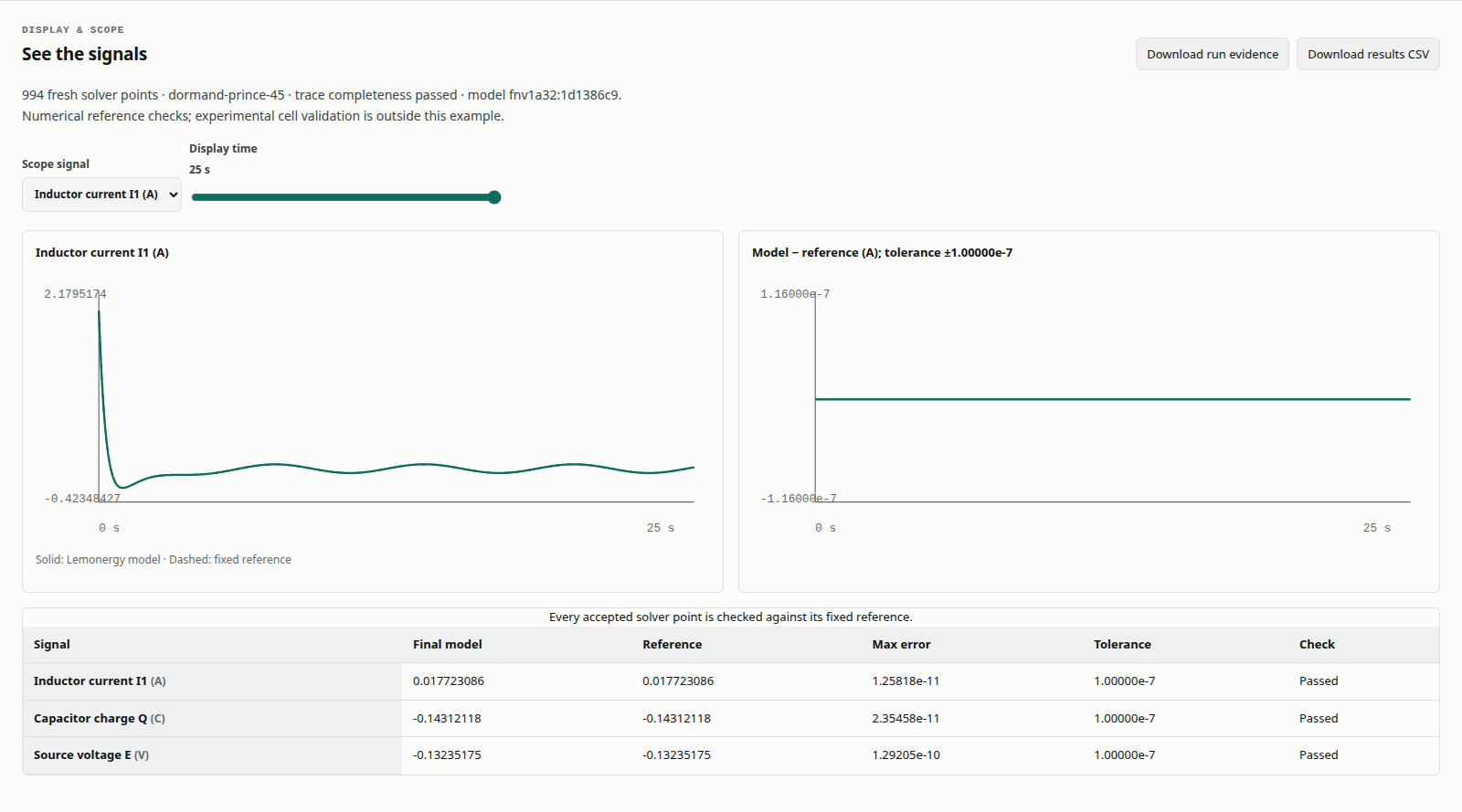
This is a real application capture. Read the table as evidence for the defined mathematical problem; a very small error against exact equations does not measure a physical component's accuracy.
Read the public result table
| Column | Meaning | How to use it |
|---|---|---|
| Signal | Compared observable and its displayed unit | Confirm which physical or logical quantity is checked |
| Final model | Last computed value of the signal | Check magnitude and units |
| Reference | Fixed-reference value at the same final instant | Compare endpoints without overlooking the rest of the trace |
| Max error | Largest absolute model/reference difference over every accepted output point | Compare with the declared tolerance |
| Tolerance | Maximum allowed absolute error for this signal | Read the exact numerical pass/fail limit |
| Check | Whether the signal satisfies its limit | Inspect every required signal, not only the first row |
The evidence JSON and historical reports also retain RMSE, the root mean square error weighting each accepted sample equally. Adaptive solvers may choose different time meshes. RMSE is not a uniform-time error integral and cannot by itself rank differently sampled solvers. A matching endpoint likewise does not establish agreement throughout the trajectory.
Use Display and Scope together
After a run, Display cards show numerical outputs at the selected retained time. Move Display time to inspect earlier points. The values change because you are inspecting a different sample, not because the model is being rerun or edited.
Choose a signal's Scope button or use Scope signal. The model/reference plot overlays the computed trajectory and the fixed reference; the neighboring plot shows their difference. An overlapping pair can conceal a small systematic error visible in the difference plot.
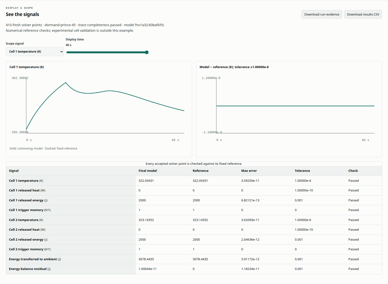
For battery pulses, inspect switching instants as well as recovery. For triggered heat propagation, inspect trigger memory, released energy and temperature. Use Download results CSV to examine exact retained sample rows rather than estimate event times from rounded axis labels.
A pass covers the complete contract
The comparator checks the case/version binding, expected block inventory and quantities, solver method/settings, strictly increasing finite times, full observation window and every required signal. Pulse cases require their switch instants; sampled thermal events require their event boundaries and latch behaviour.
A shortened trace or altered solver contract cannot pass simply because a few points agree. A failed solve or missing runtime support is not converted into a successful comparison. The public model is fixed; its settings are available for inspection under Model, method and references.
Internal thermal states use kelvin. The iron-rod comparison converts absolute temperatures to degrees Celsius; a difference has the same numerical magnitude in K and °C. The RLC model documents its explicit mapping between numerical block quantities and electrical SI units. Check the displayed unit before comparing a state value with an article table.
Investigate a failed public comparison
- Check that the expected example is selected and its model loaded successfully.
- Read the run summary and trace-completeness result, then identify any signal outside tolerance.
- Examine the first point where error appears. A step-aligned error can indicate switching or event timing; growing error can indicate a state derivative or initial value.
- Inspect the corresponding block and its incoming connections, and compare them with the article's parameter table.
- Choose Download run evidence and Download results CSV to retain the result and inputs. Selecting the same example again reloads its prepared data for a controlled rerun.
The public viewer does not allow a parameter to be changed as a troubleshooting shortcut. If you need to experiment with a variant, use Edit with Pro and keep its evidence separate from the prepared reference.
Interpret a changed model in Pro
In the Pro editor, a parameter edit changes the model while the original reference remains fixed. The rod heating exercise demonstrates this: increasing heat input changes the temperature slope, so a failed match against the unchanged original problem is expected.
Use Run blocks & compare in the Pro editor after each change. Check all signals and the full interval, then Save the variant with its matching result. Restore Load reference blocks and rerun when checking the original case. Do not widen the reference limits merely to make a different problem pass.
Separate fresh runs, saved results and historical reports
Run prepared model creates a fresh result for the supplied public graph on the current device. Download run evidence records that run; Download the model file provides the original model artifact and does not rewrite it with your fresh result.
In the Pro editor, Open can display a Saved result retained in a model file. Rechecking a retained trace is not a new solve. Run blocks & compare performs a fresh calculation of the editor's current graph.
The downloadable October 1 reports preserve their original inputs, settings and source fingerprints. Application figures carry their own capture dates and do not rewrite those historical reports. A checksum detects changed content but does not authenticate the machine or program that originally produced a file.
Interpret timing within its measured scope
| Recorded boundary | Included work |
|---|---|
| Native solve | Encode the graph, calculate all blocks and decode outputs |
| Fresh + checks | Construct the graph and run the analytical comparison as well |
| Reopen + checks | Parse and validate a saved trace without solving |
The historical reports use 20 measured warm repetitions after two warmups. File bytes are already in memory; disk access and screen rendering are outside those timings. firstRunMs is a case's first solve in an initialized process, not cold application startup. Those measurements are not timing promises for the public viewer.
The retained reports contain no executed external-tool comparison. Do not infer a cross-product speed ratio or financial saving from them. Read Collect independent comparison evidence when preparing a reproducible comparison with another implementation.