Combine conduction, thermal storage and ambient loss
Follow a rod as a hot base warms it while air removes heat. This Lemonergy example combines a conduction branch, a Thermal balance and a temperature Integrator into one feedback model. You will inspect every block, reproduce its exponential response and see how the final temperature follows from competing conductances.
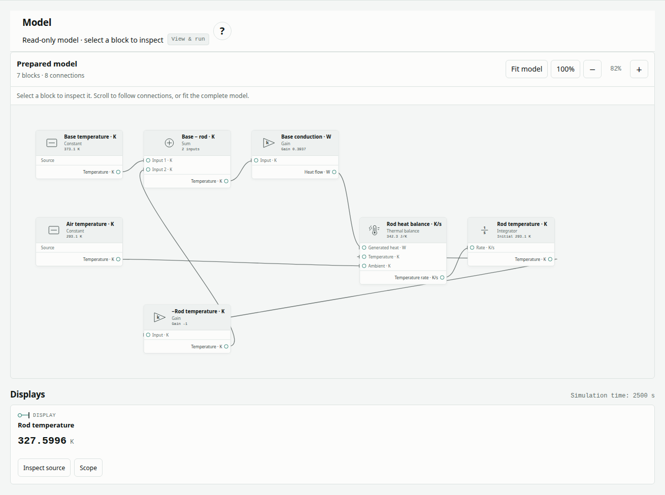
The complete mw-thermal-lumped case, reference version 1, has seven prepared blocks and eight connections, executed by the Rust/WebAssembly solver. It uses one uniform rod temperature. The conduction, convection and insulated-heating examples introduce its individual mechanisms.
Open the prepared model
Open prepared examples and choose Iron rod: lumped transient. The complete supplied model loads automatically. Choose Run prepared model to calculate a fresh result with Rust/WebAssembly, then select blocks to inspect their read-only parameters and connections. You can download the original model data for reference.
The public viewer lets you inspect, run and explore this prepared example. To change parameters, connect blocks, import a file or save an edited model, choose Edit with Pro. The Design app opens the selected example in its authenticated Pro editor; the workflow guide explains both experiences.
Define the physical balance
The rod starts at 20 °C. Its base is held at 100 °C and the air at 20 °C. A single midpoint thermal mass receives heat from the base and loses heat through lateral convection and a tip path:
A = π D² / 4
As = π D L
Cth = ρ c A L
Gbase = 2 k A / L
Gtip = 2 A k h / (L h + 2 k)
Hambient = h As + Gtip
Cth dT/dt = Gbase (Tbase − T) − Hambient (T − Tair)
The factors of two in Gbase and Gtip reflect the midpoint-to-end half-length paths in this lumped model. The tip path combines half-rod conduction and end-face convection in series. Lateral convection adds a separate parallel ambient path.
| Input or derived coefficient | Value |
|---|---|
| Diameter D / length L | 0.025 / 0.2 m |
| Density ρ | 7800 kg/m³ |
| Specific heat c | 447 J/(kg·K) |
| Conductivity k | 80.2 W/(m·K) |
| Convection coefficient h | 32.1 W/(m²·K) |
| Base / air / initial rod temperature | 100 / 20 / 20 °C |
| Cth | Approximately 342.296154563 J/K |
| Gbase | Approximately 0.393680829403 W/K |
| Hambient | Approximately 0.519376267855 W/K |
| Observation window | 0–2500 s |
All material and geometry quantities are active through these derived coefficients. They are compiled into block parameters: changing a physical dimension requires recomputing the coefficients, not only editing its descriptive label. Solver temperatures are kelvin; comparison temperatures are °C.
Inspect the full model
Select a block in the prepared diagram to inspect its read-only parameters and connections. The inventory is two Constant blocks, two Gain blocks, one Sum, one Thermal balance and one Integrator.
| Block ID · type | Parameters | Role |
|---|---|---|
base-temperature · Constant | Value 373.15 K | Fixed 100 °C base |
ambient-temperature · Constant | Value 293.15 K | Fixed 20 °C air |
negative-rod-temperature · Gain | Gain −1; temperature input/output | Negates the current rod temperature |
base-temperature-difference · Sum | 2 temperature inputs | Adds base temperature and negative rod temperature |
base-heat · Gain | Gain 0.393680829402971 W/K; temperature input, heat output | Converts base-to-rod difference to incoming heat |
temperature-rate · Thermal balance | Heat capacity 342.29615456269295 J/K; ambient conductance 0.5193762678545671 W/K | Subtracts ambient loss from incoming heat, then divides by heat capacity |
rod-temperature · Integrator | Initial 293.15 K; rate gain 1; temperature-rate input | Stores rod temperature and closes the feedback paths |
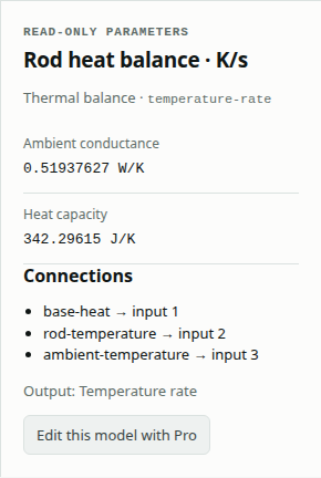
Follow rod-temperature into both negative-rod-temperature and the Thermal balance's temperature input. The negative branch forms Tbase − T, whose gain produces the generated-heat input. Air feeds the balance's ambient-temperature input. The balance sends K/s to the Integrator. These eight connections express the complete state equation; the Integrator makes the feedback a differential state path.
Run the transient comparison
- Confirm Iron rod: lumped transient is selected and loaded, with seven blocks and eight connections.
- Inspect the Integrator initial value and the three physical coefficients: Cth, Gbase and Hambient.
- Keep Dormand–Prince 4(5), the 0–2500 s window, initial step 0.01 s, minimum 1e−10 s, maximum 5 s, relative tolerance 1e−11, absolute tolerance 1e−12 and maximum 100,000 steps.
- Choose Run prepared model. Confirm Passed and trace completeness passed.
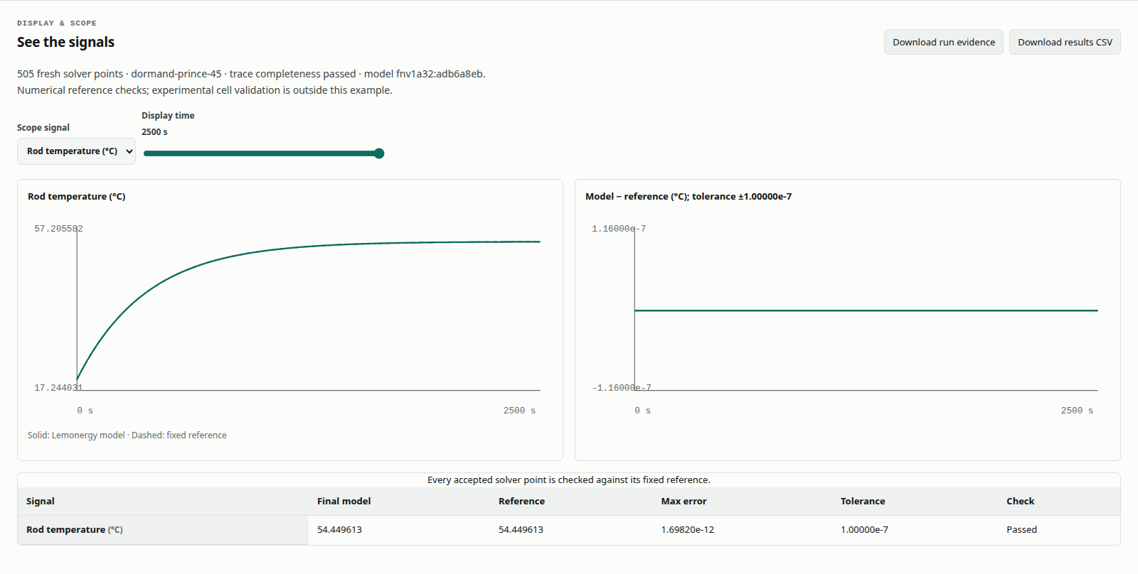
- Select Rod temperature in Scope signal and inspect both the reference overlay and native-minus-reference error plot, including the late approach to equilibrium.
- Choose Download run evidence to retain the fresh model/result comparison and Download results CSV for the sampled signals. The original model data is available under Model, method and references.
Algebraic tolerance/iteration limit is 1e−10/30; implicit tolerance/iteration limit is 1e−10/20. A comparison uses the full retained trace and original settings, not just the final temperature. See read validation results for the complete validation contract.
After the run, move Display time to inspect numerical Display outputs at retained solver times. Choose a signal’s Scope button, or use Scope signal, to view its full trajectory and reference-error plot. Scrubbing changes the inspected time, not the prepared model or its result.
Predict and interpret the result
For constant coefficients, the independent analytical reference is:
T∞ = (Gbase Tbase + Hambient Tair) / (Gbase + Hambient)
τ = Cth / (Gbase + Hambient)
T(t) = T∞ + (T0 − T∞) exp(−t/τ)
Here T∞ ≈ 54.493424833 °C and τ ≈ 374.890196452 s. The steady temperature stays below the 100 °C base because ambient loss remains nonzero. Around one time constant, the rod has completed approximately 63.2% of its total temperature rise.
| Time (s) | Analytical rod temperature (°C), rounded |
|---|---|
| 0 | 20.000000000 |
| 100 | 28.075996690 |
| 375 | 41.807719108 |
| 1000 | 52.098573869 |
| 2500 | 54.449612967 |
The 2500 s endpoint is close to equilibrium but is not the infinite-time value. The retained reference report, generated 1 October 2026 at 19:06:01 UTC, passed with 505 output points and maximum temperature error 1.698197e−12 °C against a fixed 1e−7 °C gate. This historical report is separate from the current application screenshot. The rounded checkpoints above are explanatory values; acceptance uses the full-precision reference at every retained solver time.
Try a controlled edit (Pro)
Choose Edit with Pro to open this example in the authenticated Design editor. The following changes require Pro editing. Use Run blocks & compare there to solve the edited graph; the public prepared model stays unchanged.
Select Rod heat balance · K/s and double Heat capacity from 342.29615456269295 to 684.5923091253859 J/K. Keep both conductances and boundary temperatures unchanged. This is a controlled change to storage alone: τ doubles to approximately 749.780392904 s, while the equilibrium temperature stays approximately 54.493424833 °C.
Run again. The rod warms more slowly and should fail the original transient reference despite approaching the same long-term equilibrium. Save this variant separately, then Load reference blocks and rerun to restore the case. This coefficient experiment does not represent doubling every physical rod dimension; a geometry change would also affect the conductances.
Troubleshoot feedback and equilibrium
| Symptom | What to inspect |
|---|---|
| Temperature remains at 20 °C | Check the base-difference, base-heat and Thermal balance connections |
| Temperature grows without settling | Check the −1 rod-temperature feedback and positive ambient conductance |
| Equilibrium is wrong but initial temperature agrees | Inspect both conductances and both boundary temperatures |
| Equilibrium agrees but heating is too fast | Inspect heat capacity; it determines the time constant |
| Constant offset of 273.15 | Boundary and state values must be entered in kelvin |
| Endpoint matches but comparison fails | Inspect the full trace and unchanged solver settings, not only the endpoint |
Scope, source and related reading
This is a one-state lumped approximation with fixed material properties and fixed boundary temperatures. It cannot show an axial temperature distribution, spatial fin behaviour, changing convection or radiation. Its independently derived exponential reference tests numerical implementation consistency for the stated balance, not measured physical accuracy.
The rod geometry and material inputs are attributed to MathWorks, Heat Conduction Through Iron Rod. The external application was not executed for the retained report; the transient is not an exported trace from it.
Continue with passive two-cell heat exchange for multiple coupled thermal states, battery thermal management for design context, or run, edit and save a model to build a variant. The validation examples index links all supplied models and evidence.