Reproduce a battery's pulse-voltage response
Use Lemonergy to model the immediate voltage drop and slower polarization of a cell during two discharge pulses. Inspect the prepared current waveform, ohmic branch and two first-order states, then compare terminal voltage with an independent analytical response.
The supplied case, mw-hppc-2rc reference version 1, has 14 blocks and 15 connections, executed by the Rust/WebAssembly solver. This is a forward equivalent-circuit calculation at one fixed operating point; it does not fit parameters to measured pulse data.
Open the prepared model
Open prepared examples and choose Battery pulse: two RC branches. The complete supplied model loads automatically. Choose Run prepared model to calculate a fresh result with Rust/WebAssembly, then select blocks to inspect their read-only parameters and connections. You can download the original model data for reference.
The public viewer lets you inspect, run and explore this prepared example. To change parameters, connect blocks, import a file or save an edited model, choose Edit with Pro. The Design app opens the selected example in its authenticated Pro editor; the workflow guide explains both experiences.
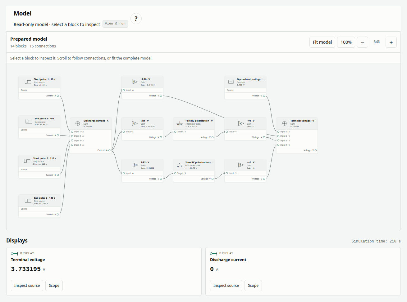
The image shows the real application canvas. The download contains the full graph, including any blocks outside the visible viewport. See run, edit and save a model for editor and file operations.
Define the cell and waveform
Positive current means discharge. Terminal voltage combines an immediate ohmic drop and two polarization voltages:
V(t) = OCV − I(t) R0 − v1(t) − v2(t)
dv1/dt = [I(t) R1 − v1(t)] / τ1
dv2/dt = [I(t) R2 − v2(t)] / τ2
v1(0) = v2(0) = 0
| Input | Value | Meaning |
|---|---|---|
| OCV | 3.7353 V | Constant open-circuit voltage |
| R0 | 0.040839 Ω | Immediate ohmic drop |
| R1 / τ1 | 0.0020343 Ω / 1.1318 s | Fast polarization branch |
| R2 / τ2 | 0.012923 Ω / 20.73 s | Slow polarization branch |
| Pulse magnitude | 6.1871 A | Positive discharge current |
| Operating-point labels | SOC 0.4; temperature 25 °C | Identify the parameter row; neither evolves |
| Initial polarization | 0 V in each branch | Fully relaxed initial model state |
Four steps produce the authored waveform: zero current for 0–10 s, 6.1871 A for 10–40 s, zero for 40–110 s, 6.1871 A for 110–140 s, then zero through 210 s. Switch values are right-continuous: at 40 s current is already zero. RC states stay continuous while the ohmic voltage changes immediately.
For each current change ΔI at time tj, the analytical branch contribution after that switch is ΔI Rk [1 − exp(−(t − tj)/τk)]. Summing all four contributions gives each reference polarization voltage independently of the model graph.
Inspect the full block inventory
Select a block in the prepared diagram to inspect its read-only parameters and connections. The inventory is four Step, two Sum, five Gain, two First-order and one Constant block.
| Block ID · type | Parameters | Connection or role |
|---|---|---|
pulse-edge-1 · Step | Before 0 A; after 6.1871 A; at 10 s | First current-sum input |
pulse-edge-2 · Step | Before 0 A; after −6.1871 A; at 40 s | Cancels first pulse |
pulse-edge-3 · Step | Before 0 A; after 6.1871 A; at 110 s | Starts second pulse |
pulse-edge-4 · Step | Before 0 A; after −6.1871 A; at 140 s | Cancels second pulse |
current · Sum | 4 inputs; current output | Adds all four steps |
ohmic-drop · Gain | −0.040839 V/A | Converts current to −I R0 |
rc1-target · Gain | 0.0020343 V/A | Current to fast branch target |
rc2-target · Gain | 0.012923 V/A | Current to slow branch target |
rc1-voltage · First-order | τ = 1.1318 s; initial 0 V | Follows rc1-target |
rc2-voltage · First-order | τ = 20.73 s; initial 0 V | Follows rc2-target |
negative-rc1 · Gain | −1 | Negates fast polarization |
negative-rc2 · Gain | −1 | Negates slow polarization |
ocv · Constant | 3.7353 V | First terminal-voltage input |
terminal-voltage · Sum | 4 inputs; voltage output | Adds OCV, ohmic drop and both negative polarization voltages |
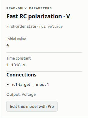
Follow current to three parallel gains. Two branches retain memory through First-order states; the ohmic branch has no state. Their outputs meet at the terminal-voltage sum. No parameter-estimation block or hidden reference simulation supplies these state values.
Run the comparison
- Confirm the loaded case is Battery pulse: two RC branches, with 14 blocks and 15 connections.
- Inspect all Step times and signs, then both First-order time constants and zero initial values.
- Keep Dormand–Prince 4(5) over 0–210 s: initial step 0.001 s, minimum 1e−10 s, maximum 0.25 s, relative tolerance 1e−10, absolute tolerance 1e−12 and maximum 100,000 steps.
- Choose Run prepared model and confirm Passed with trace completeness passed.
- Select Terminal voltage, then Discharge current in Scope signal. Examine both plots, including 10, 40, 110 and 140 s.
- Choose Download run evidence to retain the fresh model/result comparison and Download results CSV for the sampled signals. The original model data is available under Model, method and references.
Algebraic tolerance/iteration limit is 1e−10/30; implicit tolerance/iteration limit is 1e−10/20. The comparison requires every switch instant and accepted solver point. See read validation results for completeness and error checks.
After the run, move Display time to inspect numerical Display outputs at retained solver times. Choose a signal’s Scope button, or use Scope signal, to view its full trajectory and reference-error plot. Scrubbing changes the inspected time, not the prepared model or its result.
Expected voltage and current
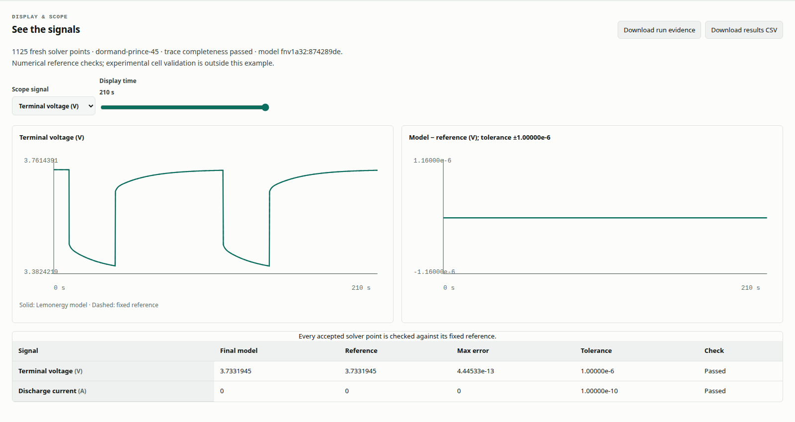
These rounded analytical checkpoints use the right-hand value at switches. They are reading checks, not replacements for the full trace comparison.
| Time (s) | Current (A) | Terminal voltage (V) | Interpretation |
|---|---|---|---|
| 0 | 0 | 3.735300000 | Both polarization states start at zero |
| 10 | 6.1871 | 3.482625023 | First immediate ohmic drop |
| 40 | 0 | 3.661565968 | Ohmic drop disappears; polarization remains |
| 110 | 6.1871 | 3.480536322 | Second pulse starts before full slow relaxation |
| 140 | 0 | 3.661074636 | Second pulse ends |
| 210 | 0 | 3.733194516 | Small slow polarization remains |
The retained reference report, generated 1 October 2026 at 19:06:01 UTC, passed with 1,125 output points. Maximum voltage error was 4.445333e−13 V against a 1e−6 V gate; current error was 0 A against a 1e−10 A gate. The historical report and current application screenshots represent separate runs.
The second pulse starts slightly lower because the slow state has not fully relaxed. Zero-current voltage recovery is a state response, not changing OCV. Both outputs must pass: a plausible voltage curve does not excuse an incorrect current waveform.
Try a controlled edit (Pro)
Choose Edit with Pro to open this example in the authenticated Design editor. The following changes require Pro editing. Use Run blocks & compare there to solve the edited graph; the public prepared model stays unchanged.
Select ohmic-drop, labeled −I·R0 · V, and change its gain from −0.040839 to −0.0449229. This increases R0 by 10%. The extra pulse drop is 6.1871 × 0.0040839 ≈ 0.0252675 V; zero-current intervals and both RC states are unchanged by this edit.
Run again. Current should still match, while voltage should fail the original gate during pulses. Save this variant under a new name. Load reference blocks and rerun to restore the supplied case. Editing a model does not rewrite its fixed reference.
Troubleshoot the response
| Symptom | Check |
|---|---|
| Current never returns to zero | End-pulse Step values must be −6.1871 A |
| Voltage rises during discharge | Check the negative ohmic gain and both −1 polarization gains |
| Voltage starts below OCV | Both First-order initial values must be 0 V |
| Only one recovery time scale | Check both target gains and First-order connections |
| Completeness fails near a switch | Restore the original settings and retain all four switch instants |
Scope, sources and related examples
OCV and parameters remain fixed. SOC evolution, hysteresis and thermal coupling are absent. The waveform is authored from a published parameter row, not replayed measured HPPC data. The numerical gate tests implementation consistency, not physical accuracy at the microvolt level. RMSE weights accepted samples equally.
The parameter row is attributed to MathWorks, Estimate Battery Model Parameters from HPPC Data. The external application was not executed for the retained report; no cross-product performance equivalence is claimed.
Continue with RLC current and charge for coupled integrators, battery thermal management for design context, or the validation examples index for the complete collection.