Integrate the temperature of an insulated thermal mass
Heat a uniform rod with a constant 18 W source and follow its temperature for 100 s. This Lemonergy example introduces a Thermal balance block and an Integrator: one calculates the temperature rate, the other stores the temperature state.
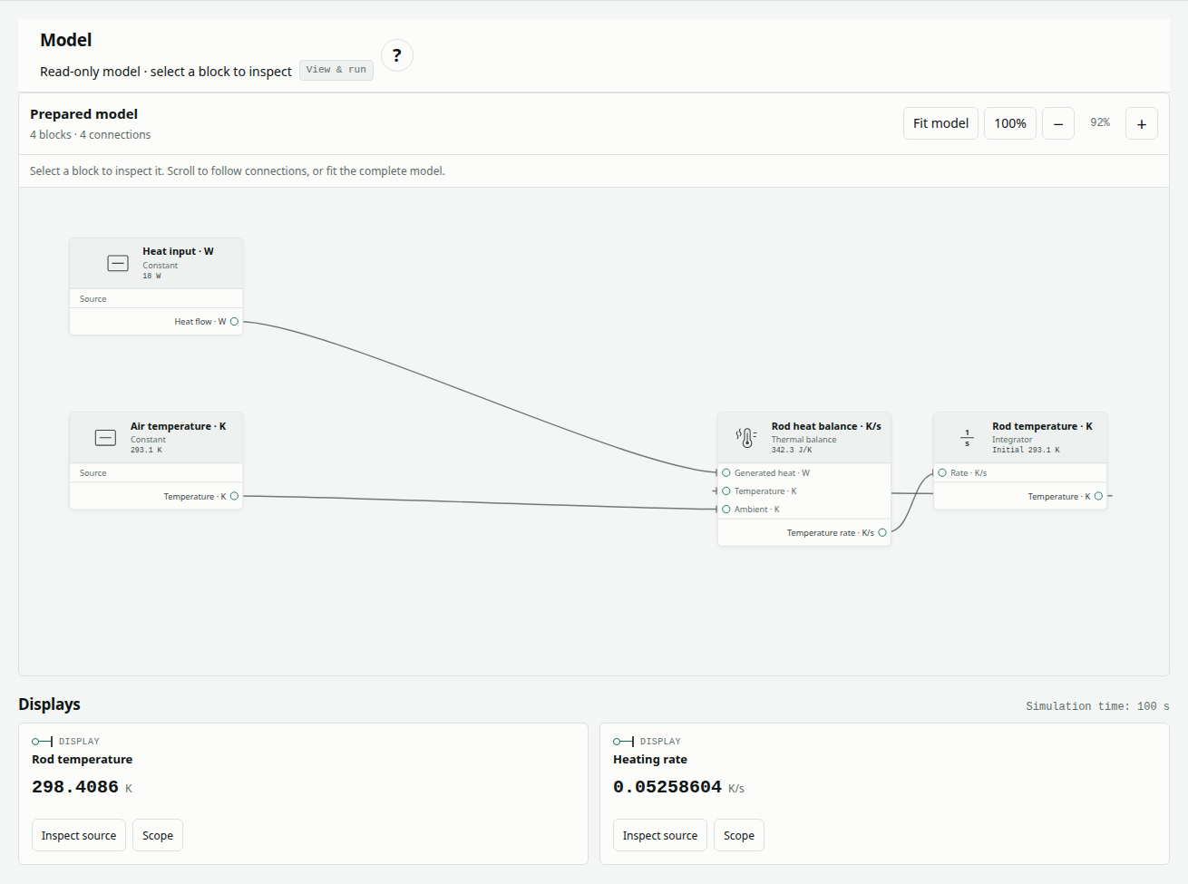
The complete mw-thermal-insulated case, reference version 1, contains four prepared blocks and four connections, executed by the Rust/WebAssembly solver. It is a useful starting point before adding the ambient losses in the lumped rod transient.
Open the prepared model
Open prepared examples and choose Iron rod: insulated heating. The complete supplied model loads automatically. Choose Run prepared model to calculate a fresh result with Rust/WebAssembly, then select blocks to inspect their read-only parameters and connections. You can download the original model data for reference.
The public viewer lets you inspect, run and explore this prepared example. To change parameters, connect blocks, import a file or save an edited model, choose Edit with Pro. The Design app opens the selected example in its authenticated Pro editor; the workflow guide explains both experiences.
Define the heat capacity and balance
The rod has one uniform temperature and no heat loss to its surroundings. Its heat capacity is mass times specific heat:
A = π D² / 4
Cth = ρ c A L
Cth dT/dt = Q
T(t) = T0 + (Q/Cth) t
| Active input or derived quantity | Value | Meaning |
|---|---|---|
| Diameter D | 0.025 m | Cross-section geometry |
| Length L | 0.2 m | Volume geometry |
| Density ρ | 7800 kg/m³ | Converts volume to mass |
| Specific heat c | 447 J/(kg·K) | Material heat storage |
| Derived heat capacity Cth | Approximately 342.296154563 J/K | Stored in the Thermal balance parameter |
| Initial temperature T0 | 20 °C = 293.15 K | Integrator initial state |
| Heat input Q | 18 W | Constant energy input per second |
| Ambient conductance | 0 W/K | No environmental heat loss |
| Observation window | 0–100 s | Authored transient interval |
The source metadata also carries conductivity 80.2 W/(m·K) and convection coefficient 32.1 W/(m²·K), but neither is active in this insulated graph. The material and geometry values are already combined in Cth; changing a written geometry label does not change that live block parameter.
The solver stores temperature in kelvin and rate in K/s. The comparison displays temperature in °C. A rise of 1 K is a rise of 1 °C, so converting the absolute temperature does not alter the slope.
Inspect the blocks and feedback path
Select a block in the prepared diagram to inspect its read-only parameters and connections. The full inventory is two Constant blocks, one Thermal balance and one Integrator.
| Block ID · type | Parameters | Connection and role |
|---|---|---|
imposed-heat · Constant | Value 18 W; heat output | Feeds the generated-heat input of Thermal balance |
ambient-temperature · Constant | Value 293.15 K; temperature output | Feeds the ambient-temperature input |
temperature-rate · Thermal balance | Heat capacity 342.29615456269295 J/K; ambient conductance 0 W/K | Returns [Q − H(T − Tair)]/Cth in K/s |
rod-temperature · Integrator | Initial 293.15 K; rate gain 1; temperature-rate input | Integrates the rate and feeds temperature back to the balance |
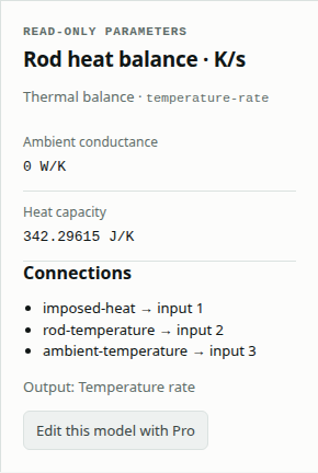
The temperature feedback and ambient input are connected even though H is zero. They make the Thermal balance interface explicit; the ambient source has no effect while the conductance remains zero. The Integrator breaks the state feedback path, so the model does not require an instantaneous algebraic loop.
Run both temperature and rate comparisons
- Confirm Iron rod: insulated heating is selected and loaded, with four blocks and four connections.
- Inspect the Thermal balance's heat capacity and zero conductance, then the Integrator's 293.15 K initial value.
- Keep Dormand–Prince 4(5), start 0 s, end 100 s, initial step 0.01 s, minimum 1e−10 s, maximum 5 s, relative tolerance 1e−11 and absolute tolerance 1e−12. Maximum steps is 100,000.
- Choose Run prepared model. Confirm Passed and trace completeness passed.
- In Scope signal, inspect Rod temperature, then Heating rate. Temperature rises linearly; rate stays constant. Examine both error plots.
- Choose Download run evidence to retain the fresh model/result comparison and Download results CSV for the sampled signals. The original model data is available under Model, method and references.
Algebraic tolerance/iteration limit is 1e−10/30; implicit tolerance/iteration limit is 1e−10/20. See read validation results if the traces look plausible but the contract or a gate fails.
After the run, move Display time to inspect numerical Display outputs at retained solver times. Choose a signal’s Scope button, or use Scope signal, to view its full trajectory and reference-error plot. Scrubbing changes the inspected time, not the prepared model or its result.
Expected temperature rise
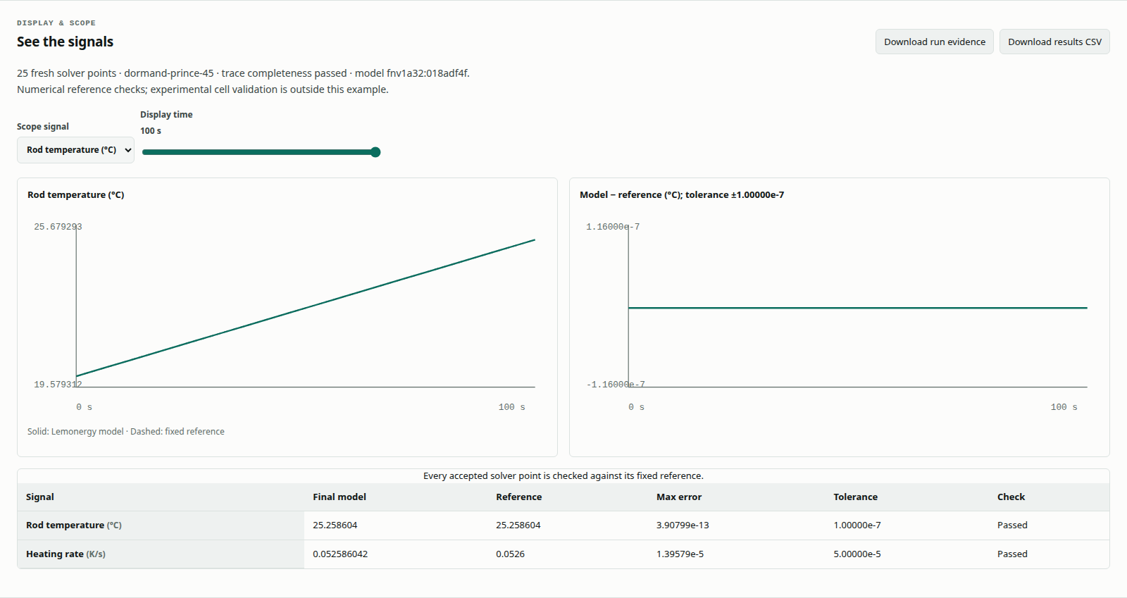
The calculated rate is 18/342.29615456269295 ≈ 0.052586042116 K/s. These rounded analytical checkpoints make the expected trajectory readable:
| Time (s) | Temperature (°C) | Added energy Q t (J) |
|---|---|---|
| 0 | 20.000000000 | 0 |
| 25 | 21.314651053 | 450 |
| 50 | 22.629302106 | 900 |
| 100 | 25.258604212 | 1800 |
Multiplying the final rise by Cth returns 1800 J. This is a balance check derived from the model; the example compares temperature and rate rather than exporting a separate energy-residual signal.
The retained reference report, generated 1 October 2026 at 19:06:01 UTC, passed with 25 output points. Its temperature maximum error was 3.907985e−13 °C against the 1e−7 °C gate. The rate is compared with the printed value 0.0526 K/s, giving a maximum difference of 1.395788e−5 K/s against a 0.00005 K/s gate. Historical report values are distinct from the fresh application capture.
The different errors have different meanings: temperature uses an independently derived full-precision trajectory, while rate uses a rounded printed scalar. The rate discrepancy is expected rounding, not accumulating numerical drift. The display checkpoints above are also rounded and are not acceptance thresholds.
Try a controlled edit (Pro)
Choose Edit with Pro to open this example in the authenticated Design editor. The following changes require Pro editing. Use Run blocks & compare there to solve the edited graph; the public prepared model stays unchanged.
Select Heat input · W and change its value from 18 to 19.8 W. The input rises 10%, so the predicted rate becomes approximately 0.057844646328 K/s and the 100 s temperature becomes approximately 25.784464633 °C.
Run again. Both original comparisons should fail because the reference remains fixed to 18 W. Save the variant separately, then Load reference blocks and rerun to restore the case. As another physical interpretation, increasing Cth while keeping Q fixed would reduce the slope; edit the Thermal balance parameter when exploring that effect.
Troubleshoot the transient
| Symptom | What to inspect |
|---|---|
| Temperature remains constant | Confirm heat reaches Thermal balance and rate reaches the Integrator |
| Temperature approaches a plateau | Ambient conductance must be zero for this case |
| Correct slope but wrong starting point | Integrator initial value must be 293.15 K |
| Temperature rises much too quickly | Heat capacity is in J/K and heat input is in W, not kW |
| Rate differs slightly from 0.0526 | Expected: the reference rate is printed to four decimal places |
Scope, source and next steps
Uniform temperature and constant material properties are assumptions. There is no spatial field, radiation, conduction to a support or measured rod trace. The 100 s horizon is authored. Numerical agreement verifies this balance and its integration for the stated settings, not physical accuracy under arbitrary heating conditions.
The rod inputs and rounded heating-rate answer are attributed to MathWorks, Heat Conduction Through Iron Rod. The transient is independently derived from the heat balance; the external application was not executed for the retained report.
Continue with the lumped transient to combine heat storage and losses, or passive heat exchange between two cells to examine two interacting thermal states and an explicit energy residual. The validation index links the full collection.