Solve coupled current and charge equations
Explore a prepared RLC equation model in Lemonergy, inspect its feedback paths and compare current, capacitor charge and source voltage with a fixed analytical solution. Ordinary Gain, Sum and Integrator blocks form this coupled dynamic system, including the oscillator that generates its input.
The complete example is mw-rlc, reference version 1: 12 prepared blocks, 15 connections and three compared signals, executed by the Rust/WebAssembly solver. Familiarity with derivatives and feedback is useful; no external numerical application is needed.
Open the prepared model
Open prepared examples and choose RLC circuit: current and charge. The complete supplied model loads automatically. Choose Run prepared model to calculate a fresh result with Rust/WebAssembly, then select blocks to inspect their read-only parameters and connections. You can download the original model data for reference.
The public viewer lets you inspect, run and explore this prepared example. To change parameters, connect blocks, import a file or save an edited model, choose Edit with Pro. The Design app opens the selected example in its authenticated Pro editor; the workflow guide explains both experiences.
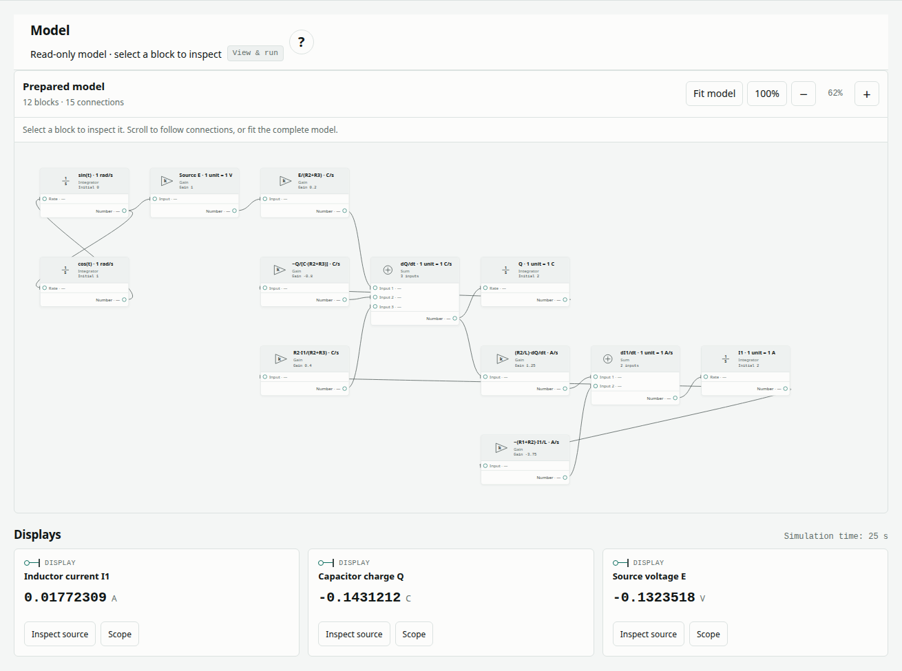
The screenshot shows the application canvas; the download contains the complete graph, including blocks outside the visible viewport. See run, edit and save a model for the general editor workflow.
Define the equations and units
The forcing voltage is E(t) = sin(t) V. The coupled equations are:
dQ/dt  = [E − Q/C + R2 I1] / (R2 + R3)
dI1/dt = (R2/L) dQ/dt − [(R1 + R2)/L] I1
| Physical parameter | Value | Where it enters |
|---|---|---|
| R1 / R2 / R3 | 4 / 2 / 3 Ω | Current damping and charge-rate coefficients |
| Inductance L | 1.6 H | Current-rate coefficients |
| Capacitance C | 0.25 F | Charge feedback |
| Initial I1 / Q | 2 A / 2 C | Current and charge integrator initial values |
| Source amplitude | 1 V | Source E gain |
| Angular frequency | 1 rad/s | Paired sine/cosine integrator rate gains |
| Observation window | 0–25 s | Complete comparison interval |
The catalog lacks charge and current-rate quantity types. This executable model therefore uses dimensionless block ports with an explicit SI numerical mapping: one current unit is 1 A, one charge unit is 1 C and one voltage unit is 1 V; time is seconds. Charge-rate and current-rate numbers represent C/s and A/s. The editor does not enforce those electrical dimensions for this case.
Inspect every block and connection
Select a block in the prepared diagram to inspect its read-only parameters and connections. All blocks below are present in the supplied model.
| Block ID · type | Parameter values | Role and connection |
|---|---|---|
sin-time · Integrator | Initial 0; rate gain 1 | Integrates cos-time to generate sin(t) |
cos-time · Integrator | Initial 1; rate gain −1 | Integrates sin-time with a negative sign to generate cos(t) |
input-voltage · Gain | Gain 1 | Takes sin-time; produces E |
charge-input · Gain | Gain 0.2 | E/(R2 + R3); feeds charge-rate input 1 |
charge-feedback · Gain | Gain −0.8 | Takes Q; produces −Q/[C(R2 + R3)] |
current-to-charge · Gain | Gain 0.4 | Takes I1; produces R2 I1/(R2 + R3) |
charge-rate · Sum | 3 inputs | Adds the preceding three charge-rate terms |
charge · Integrator | Initial 2; rate gain 1 | Integrates charge-rate to produce Q |
charge-to-current · Gain | Gain 1.25 | Multiplies charge-rate by R2/L |
current-feedback · Gain | Gain −3.75 | Multiplies I1 by −(R1 + R2)/L |
current-rate · Sum | 2 inputs | Adds charge-to-current and current-feedback |
current · Integrator | Initial 2; rate gain 1 | Integrates current-rate to produce I1 |
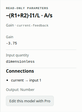
The oscillator is a feedback pair of states, not a precomputed trace. Likewise, charge and current return their states to the rate equations. Integrators make these differential feedback paths executable without an instantaneous algebraic loop. The physical component values are represented by the listed gains; there are no hidden dedicated electrical components to locate.
Run and examine all three signals
- Check that the selected and loaded case are both RLC circuit: current and charge.
- Inspect the four integrator initial values: sine 0, cosine 1, charge 2 and current 2.
- Keep the solver settings: Dormand–Prince 4(5), initial step 0.001 s, minimum step 1e−10 s, maximum step 0.05 s, relative tolerance 1e−10 and absolute tolerance 1e−12. The maximum step count is 100,000.
- Choose Run prepared model. Confirm Passed and a complete 0–25 s trace.
- In Scope signal, examine Inductor current I1, Capacitor charge Q and Source voltage E individually. Inspect both the overlay and native-minus-reference error plot.
- Choose Download run evidence to retain the fresh model/result comparison and Download results CSV for the sampled signals. The original model data is available under Model, method and references.
The retained algebraic tolerance/iteration limit is 1e−10/30; the implicit tolerance/iteration limit is 1e−10/20. Changing solver settings changes the comparison contract. See reading validation results for completeness checks and error metrics.
After the run, move Display time to inspect numerical Display outputs at retained solver times. Choose a signal’s Scope button, or use Scope signal, to view its full trajectory and reference-error plot. Scrubbing changes the inspected time, not the prepared model or its result.
Expected numerical results
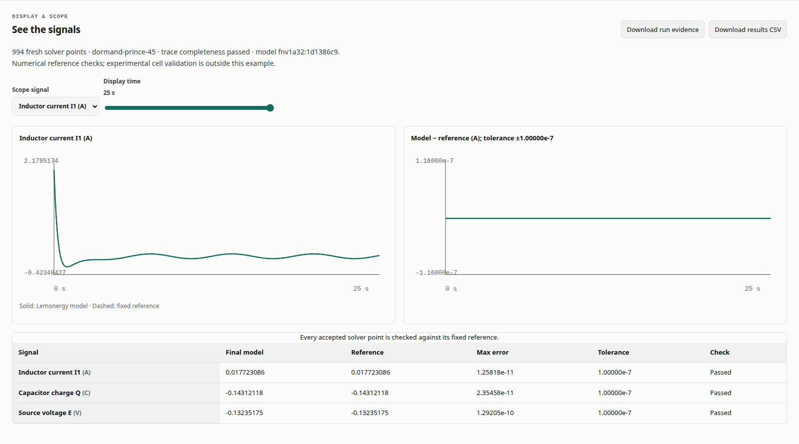
The initial electrical states decay while sinusoidal forcing remains. These rounded checkpoints evaluate the fixed analytical reference; the comparison uses its full precision at every accepted output time.
| Time (s) | I1 (A) | Q (C) | E (V) |
|---|---|---|---|
| 0 | 2.000000000 | 2.000000000 | 0.000000000 |
| 1 | −0.243943221 | 1.011384740 | 0.841470985 |
| 5 | −0.049607886 | −0.124836727 | −0.958924275 |
| 10 | −0.047628898 | 0.047029858 | −0.544021111 |
| 25 | 0.017723086 | −0.143121184 | −0.132351750 |
The retained reference report, generated 1 October 2026 at 19:06:01 UTC, passed with 994 output points. Maximum absolute errors were 1.258182e−11 A for I1, 2.354578e−11 C for Q and 1.292054e−10 V for E. Each fixed gate is 1e−7 in its signal's displayed unit. These historical metrics are separate from the fresh application run illustrated above.
Checking E independently matters: a plausible current trace could conceal an incorrectly wired oscillator. Negative current or charge is allowed by these equations and initial conditions; it is not itself a numerical failure.
Try a controlled edit (Pro)
Choose Edit with Pro to open this example in the authenticated Design editor. The following changes require Pro editing. Use Run blocks & compare there to solve the edited graph; the public prepared model stays unchanged.
Change only Gain on input-voltage from 1 to 1.1. This increases the sine amplitude to 1.1 V while preserving initial current and charge. Run again: the source and driven electrical states should differ from the original reference, so the original comparison should fail. A failed reference match is expected for an intentionally changed model.
Save the edited model under a new name, then choose Load reference blocks and rerun to restore the supplied case. If changing a physical resistance or capacitance instead, update every affected coefficient in the equations; changing one coefficient alone generally represents a different mathematical system.
Troubleshoot the model
| Symptom | What to inspect |
|---|---|
| E grows instead of oscillating | cos-time rate gain must be −1; both oscillator connections must be present |
| Wrong initial point | Initial values on charge and current must both be 2 |
| Charge decays incorrectly | Confirm the −0.8 charge feedback and 0.4 current-to-charge gains |
| Current differs while E agrees | Check gains 1.25 and −3.75 and both inputs to current-rate |
| Trace is incomplete | Restore reference settings and the full 0–25 s window; retain every accepted point |
Scope, sources and related reading
This verifies a numerical equation graph against a retained closed-form solution. It does not validate a dedicated electrical-network compiler, symbolic solver or physical circuit. The reference does not read edited parameters. The maximum-error gate applies to the full trace; RMSE weights accepted samples equally rather than integrating error uniformly in time.
The equations and analytical solution are attributed to MathWorks, Solve Differential Equations of RLC Circuit Using Laplace Transform. The external application was not executed for the retained report. Agreement for this specified problem does not establish general product equivalence.
Continue with the two-branch battery pulse model to compare exponential polarization states, or the lumped thermal transient to apply state feedback to heat flow. The validation examples index links the complete collection and evidence.