Exchange heat between two thermal masses
Heat that leaves one body must enter the other. In this example, equal thermal masses begin at 400 K and 300 K and exchange heat through a conductive link. You will inspect the connected model, reproduce both temperature histories and check conservation with an independent energy residual.
The supplied model is tr-two-cell-exchange, reference version 1. Its 35 prepared blocks and 42 connections run in Lemonergy's Rust/WebAssembly engine. Start here before adding a finite heat pulse or sampled propagation logic.
Open the prepared model
Open prepared examples and choose Two cells: passive heat exchange. The complete supplied model loads automatically. Choose Run prepared model to calculate a fresh result with Rust/WebAssembly, then select blocks to inspect their read-only parameters and connections. You can download the original model data for reference.
The public viewer lets you inspect, run and explore this prepared example. To change parameters, connect blocks, import a file or save an edited model, choose Edit with Pro. The Design app opens the selected example in its authenticated Pro editor; the workflow guide explains both experiences.
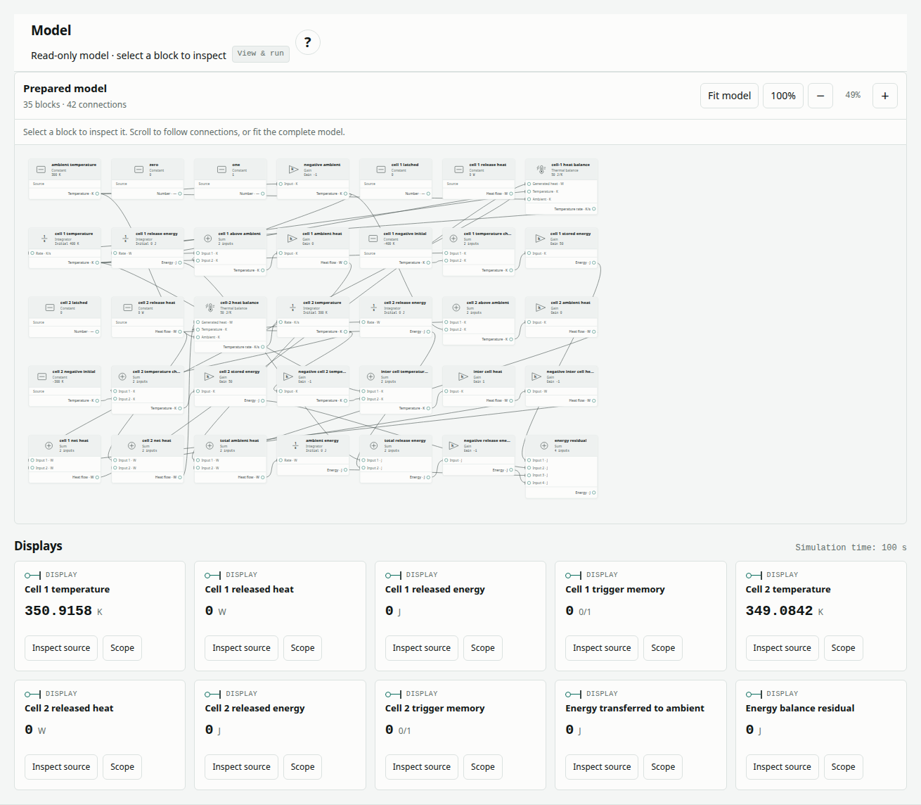
The energy-accounting branches are part of the verification. They track heat and energy without adding physical cells.
Define the thermal problem
Each cell has one uniform temperature and a constant heat capacity. Positive link heat flows from cell 1 to cell 2:
q12 = G (T1 − T2)
C dT1/dt = −q12
C dT2/dt = +q12
Adding these balances shows that the mean temperature stays at 350 K. The temperature difference decays with time constant C/(2G) = 25 s. The independent analytical solution is:
T1(t) = 350 + 50 exp(−0.04t) K
T2(t) = 350 − 50 exp(−0.04t) K
| Quantity | Value | Meaning |
|---|---|---|
| Heat capacity C | 50 J/K per cell | Stored heat per kelvin of change |
| Initial T1, T2 | 400 K, 300 K | Integrator initial values |
| Link conductance G | 1 W/K | Link heat per temperature difference |
| Ambient conductance H | 0 W/K per cell | No heat leaves the pair |
| Ambient temperature | 300 K | Has no effect while H is zero |
| Release power | 0 W | No active release or trigger |
| Observation window | 0–100 s | Four exchange time constants |
Inspect the blocks and parameters
Select a block in the prepared diagram to inspect its read-only parameters and connections. The inventory is 9 Constant, 9 Gain, 10 Sum, 5 Integrator and 2 Thermal balance blocks. This passive example needs no trigger, latch or timer.
| Block or group | Parameter or connection | Purpose |
|---|---|---|
ambient-temperature, zero, one · Constants | 300 K, 0, 1 | Supply ambient and retained logic constants; zero/one are inactive in this passive case |
negative-ambient · Gain | Gain −1 | Form −Ta for ambient-loss accounting |
cell-1-latched, cell-2-latched · Constants | Value 0 | Expose inactive trigger-memory signals without adding latch blocks |
cell-1-release-heat, cell-2-release-heat · Constants | Value 0 W | Supply zero released heat |
cell-1-temperature, cell-2-temperature · Integrator | Initial 400 / 300 K; rate gain 1; temperature-rate input | Store the two temperatures |
cell-1-temperature-rate, cell-2-temperature-rate · Thermal balance | Heat capacity 50 J/K; ambient conductance 0 W/K | Divide net heat by C |
negative-cell-2-temperature · Gain | Gain −1 | Form −T2 for the link difference |
inter-cell-temperature-difference · Sum | T1 plus −1 times T2 | Form T1 − T2 |
inter-cell-heat · Gain | Gain 1; temperature input, heat output | Calculate q12 |
negative-inter-cell-heat · Gain | Gain −1 | Apply the opposite heat flow to cell 1 |
cell-1-net-heat, cell-2-net-heat · Sum | Release heat plus signed link heat | Feed the Thermal balance generated-heat ports |
cell-1-release-energy, cell-2-release-energy · Integrators | Initial 0 J; gain 1; integrate zero release heat | Confirm no introduced heat |
cell-1-above-ambient, cell-2-above-ambient · Sums | Two inputs each: Ti and −Ta | Form ambient temperature differences |
cell-1-ambient-heat, cell-2-ambient-heat · Gains | Gain 0 W/K | Produce zero ambient heat loss |
cell-1-negative-initial, cell-2-negative-initial · Constants | −400 K, −300 K | Supply negative initial temperatures |
cell-1-temperature-change, cell-2-temperature-change · Sums | Two inputs each: Ti and −Ti(0) | Calculate temperature changes |
cell-1-stored-energy, cell-2-stored-energy · Gains | Gain 50 J/K | Calculate stored-energy changes |
total-ambient-heat · Sum; ambient-energy · Integrator | Two inputs; initial 0 J, gain 1 | Track environmental loss |
total-release-energy · Sum; negative-release-energy · Gain | Two inputs; gain −1 | Form the negative release total |
energy-residual · Sum | Stored changes + ambient energy − released energy | Check complete-pair conservation |
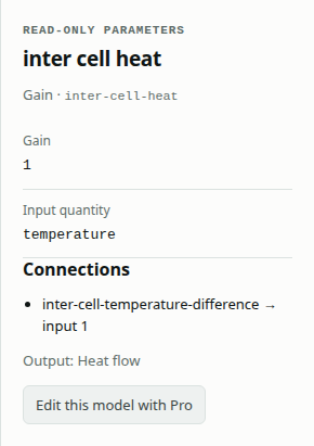
The energy check uses changes in stored energy. The initially hot cell therefore does not create an artificial residual, and link heat cancels when the two balances are added.
Run the reference comparison
- Confirm the loaded binding: 35 blocks, 42 connections and a 0–100 s window.
- Keep the reference solver settings shown below. Changing the settings changes the verification contract.
- Choose Run prepared model. Confirm Passed and trace completeness passed.
- In Scope signal, inspect Cell 1 temperature, then Cell 2 temperature, using both the overlay and native-minus-reference plot.
- Inspect Energy balance residual, both release-energy signals and Energy transferred to ambient. They should stay zero within their gates.
- Choose Download run evidence to retain the fresh model/result comparison and Download results CSV for the sampled signals. The original model data is available under Model, method and references.
| Solver setting | Reference value |
|---|---|
| Method | Dormand–Prince 4(5) |
| Initial / minimum / maximum step | 0.001 / 1e−10 / 0.1 s |
| Relative / absolute tolerance | 1e−11 / 1e−12 |
| Maximum steps | 100,000 |
| Algebraic tolerance / iteration limit | 1e−10 / 30 |
| Implicit tolerance / iteration limit | 1e−10 / 20 |
After the run, move Display time to inspect numerical Display outputs at retained solver times. Choose a signal’s Scope button, or use Scope signal, to view its full trajectory and reference-error plot. Scrubbing changes the inspected time, not the prepared model or its result.
Understand the result
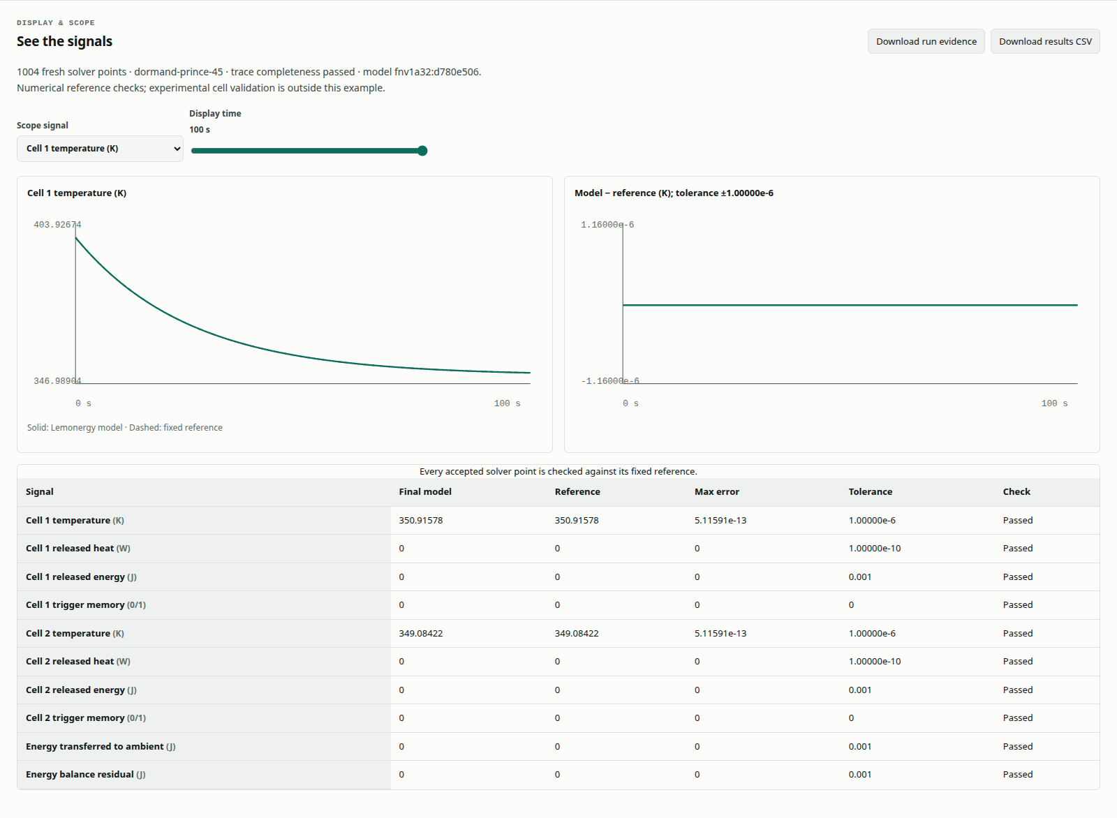
The hot cell cools while the cold cell warms. At 100 s they have not quite reached 350 K: exponential equilibration is asymptotic. These analytical checkpoints are rounded for reading, not used as acceptance tolerances:
| Time (s) | T1 (K) | T2 (K) | Mean (K) |
|---|---|---|---|
| 0 | 400.000000 | 300.000000 | 350 |
| 25 | 368.393972 | 331.606028 | 350 |
| 50 | 356.766764 | 343.233236 | 350 |
| 100 | 350.915782 | 349.084218 | 350 |
The retained thermal report, generated 1 October 2026 at 18:52:33 UTC, passed with 1,004 output points. Maximum temperature error was approximately 5.12e−13 K for either cell, and maximum energy residual was 0 J. These historical values are distinct from a new run shown in the current interface screenshots.
Fixed gates are 1e−6 K for temperature, 1e−10 W for release heat, 1e−3 J for each energy signal and exactly zero trigger-memory error. A pass also requires the original settings, the full window, every accepted point and finite values for every block.
Try a controlled change (Pro)
Choose Edit with Pro to open this example in the authenticated Design editor. The following changes require Pro editing. Use Run blocks & compare there to solve the edited graph; the public prepared model stays unchanged.
Change only Gain on inter-cell-heat from 1 to 2. The predicted time constant becomes 12.5 s, so the cells approach their mean faster. Their mean should still stay at 350 K and the energy residual should remain near zero because the same link feeds both cells with opposite signs.
Run again. The temperature comparison should fail against the unchanged 1 W/K reference; this is the expected consequence of the changed input. Save the variant separately, then reload the reference blocks and rerun. Do not widen the original gates to accommodate a different model.
Troubleshoot and assess the scope
| Observation | Check |
|---|---|
| Both temperatures move in the same direction | The −1 gain in the cell-1 link branch and both net-heat connections |
| The mean drifts toward 300 K | Both ambient conductances must be zero |
| Correct temperatures but a large residual | Initial-temperature subtraction and the signs of stored, ambient and released energy |
| Run is unavailable | Wait for the prepared model to finish loading; choose the example again if loading fails |
| Downloads are unavailable | Complete a fresh run of the selected prepared model first |
This is a synthetic lumped-network check with constant properties, no spatial temperature field and no heat-release event. It establishes consistency with the equations, not measured cell behavior or safety performance.
References and related reading
The retained thermal report preserves the historical numerical evidence. External architecture documentation among this article's sources provides background; MATLAB/Simscape was not executed for that retained check. Continue with thermal propagation verification, battery thermal management and read validation results.