Calculate heat lost from a cylindrical surface
Use Lemonergy to calculate convection from a uniform-temperature rod into cooler air. This example builds a temperature difference, converts it to heat flow through a surface conductance and checks the result against a published scalar answer.
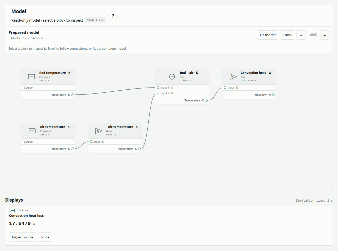
The executable mw-thermal-convection case, reference version 1, contains five prepared blocks and four connections. It runs through the Rust/WebAssembly solver. Start here to understand a convection coefficient before using ambient losses in a lumped thermal transient.
Open the prepared model
Open prepared examples and choose Iron rod: cylindrical convection. The complete supplied model loads automatically. Choose Run prepared model to calculate a fresh result with Rust/WebAssembly, then select blocks to inspect their read-only parameters and connections. You can download the original model data for reference.
The public viewer lets you inspect, run and explore this prepared example. To change parameters, connect blocks, import a file or save an edited model, choose Edit with Pro. The Design app opens the selected example in its authenticated Pro editor; the workflow guide explains both experiences.
Define the surface heat transfer
The model assumes the whole rod surface stays at 55 °C while air stays at 20 °C. Its lateral cylindrical area is As = π D L. Heat lost to air is:
ΔT = Trod − Tair
Hsurface = h As = h π D L
Q = Hsurface ΔT
| Active input or derived quantity | Value | Meaning |
|---|---|---|
| Diameter D | 0.025 m | Diameter of lateral surface |
| Length L | 0.2 m | Length exposed to air |
| Convection coefficient h | 32.1 W/(m²·K) | Fixed coefficient; not calculated from flow |
| Rod temperature | 55 °C = 328.15 K | Fixed hot source |
| Air temperature | 20 °C = 293.15 K | Fixed ambient source |
| Lateral surface area As | Approximately 0.015707963268 m² | Excludes the two circular ends |
| Surface conductance Hsurface | Approximately 0.504225620901 W/K | Stored in the final Gain block |
| Temperature difference | 35 K | Equal to a difference of 35 °C |
Density 7800 kg/m³, specific heat 447 J/(kg·K) and conductivity 80.2 W/(m·K) remain in the shared rod metadata but do not participate in this graph. Neither thermal mass nor axial conduction is active. The separate conduction example uses the conductivity.
Inspect the blocks and their connections
Select a block in the prepared diagram to inspect its read-only parameters and connections. There are two Constant blocks, two Gain blocks and one Sum.
| Block ID · type | Parameter values | Role |
|---|---|---|
uniform-temperature · Constant | Value 328.15 K; temperature output | Positive input to the temperature difference |
ambient-temperature · Constant | Value 293.15 K; temperature output | Feeds the negative-ambient gain |
negative-ambient · Gain | Gain −1; temperature input/output | Negates air temperature |
temperature-difference · Sum | 2 inputs; temperature output | Adds rod temperature and negative air temperature |
convection-heat · Gain | Gain 0.5042256209011619 W/K; temperature input, heat output | Converts the difference to outward heat flow |
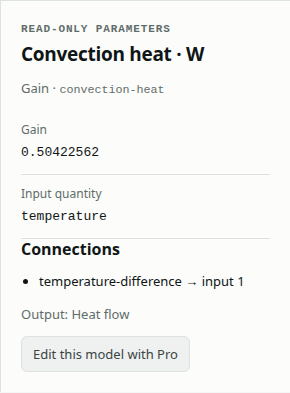
Connect ambient-temperature to negative-ambient, then to the second sum input. Connect uniform-temperature directly to the first sum input. Finally, connect the sum to convection-heat. The temperature difference travels through the catalog's temperature-quantity port; subtracting the two kelvin sources removes their common offset.
No Integrator is missing: both temperatures are imposed, so this example returns a constant heat flow. It does not cool the rod over time.
Run the comparison
- Confirm the selected and loaded case is Iron rod: cylindrical convection, with five blocks and four connections.
- Check the source values 328.15 K and 293.15 K and the −1 ambient gain.
- Keep the 0–1 s observation interval. The retained configuration is Dormand–Prince 4(5), initial step 0.01 s, minimum 1e−10 s, maximum 5 s, relative tolerance 1e−11, absolute tolerance 1e−12 and maximum 100,000 steps.
- Choose Run prepared model. Confirm Passed and trace completeness passed.
- In Scope signal, inspect Convection heat loss, the reference overlay and the error plot.
- Choose Download run evidence to retain the fresh model/result comparison and Download results CSV for the sampled signals. The original model data is available under Model, method and references.
The algebraic tolerance/iteration limit is 1e−10/30 and implicit tolerance/iteration limit is 1e−10/20. The two endpoint observations describe a constant result, not a one-second cooling experiment. See read validation results for interpreting gates and trace completeness.
After the run, move Display time to inspect numerical Display outputs at retained solver times. Choose a signal’s Scope button, or use Scope signal, to view its full trajectory and reference-error plot. Scrubbing changes the inspected time, not the prepared model or its result.
Expected heat loss
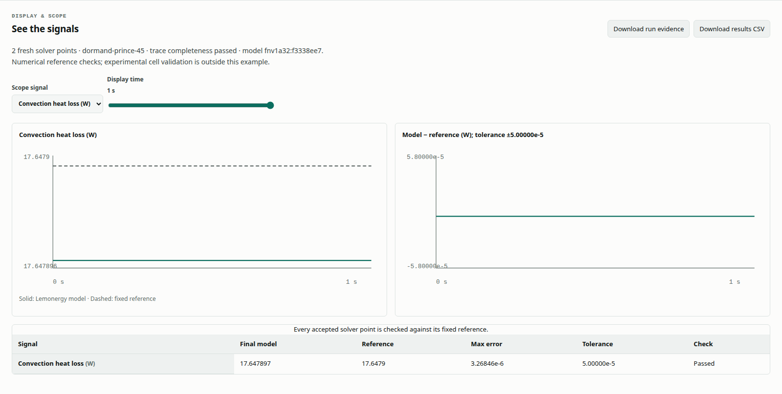
Substituting the inputs gives Q = 0.5042256209011619 × 35 ≈ 17.647896732 W.
| Quantity | Value |
|---|---|
| Calculated lateral heat loss | Approximately 17.647896732 W |
| Printed reference heat loss | 17.6479 W |
| Absolute rounding difference | Approximately 0.00000326846 W |
| Fixed maximum absolute error gate | 0.00005 W |
The retained reference report, generated 1 October 2026 at 19:06:01 UTC, passed with two output points and maximum error 3.268459e−6 W. That report and the fresh application screenshots are separate runs. The gate is half the reference answer's last printed decimal, not an estimate of convection-model uncertainty.
Positive Q means heat leaves the hotter rod. If both source temperatures were equal, this relation would return zero heat. Reversing their difference would reverse the direction of heat flow. These checks help distinguish a sign or wiring error from a numerical issue.
Try a controlled edit (Pro)
Choose Edit with Pro to open this example in the authenticated Design editor. The following changes require Pro editing. Use Run blocks & compare there to solve the edited graph; the public prepared model stays unchanged.
Select Rod temperature · K and change its value from 328.15 to 338.15 K, representing 65 °C. With air unchanged, the difference becomes 45 K and the new heat loss should be approximately 22.690152941 W. The original 17.6479 W comparison should fail because the physical input changed.
Save the variant under a new name, then Load reference blocks and rerun to restore the original. If changing diameter, length or h instead, recompute the final gain h π D L; those values are compiled into the coefficient and are not separate parameter blocks on this canvas.
Troubleshoot units and boundaries
| Symptom | What to inspect |
|---|---|
| Negative heat with a hotter rod | Check the subtraction order and negative-ambient gain |
| An unexpectedly large heat flow | Do not add absolute temperatures; the gain needs their difference |
| A nearly correct result fails | Check the exact unrounded gain and unchanged source values |
| No temperature decay appears | Expected: rod and air temperatures are fixed sources |
| Heat loss includes end faces | This graph uses lateral area only; end losses need a separate model term |
Scope, source and related examples
Uniform rod temperature, fixed air temperature and constant h are assumptions. This model does not predict a flow field, radiation, thermal storage or evolving surface temperature. Passing checks the numerical implementation of the stated relation, not measured physical accuracy or a complete thermal design.
The rod inputs and printed scalar are attributed to MathWorks, Heat Conduction Through Iron Rod. The external application was not executed for the retained report.
Compare steady axial conduction, insulated heating and the lumped rod transient to see how each mechanism changes the graph. The validation examples index links the complete model collection.