Engineering review · items 4, 5 and 6
The remaining implementation changes are now available in the controls above. The table distinguishes working calculations from the vehicle measurements still needed to validate them.
| Item | Implemented and checked | Evidence still needed |
|---|---|---|
| 4 · Gas storage | Manufacturer cylinder dimensions and service pressure, integer count, cylinder/valve/mount mass, three packing orientations and a bay-limited loading action. | Actual vehicle bay CAD, real-gas density, installed vessel approval, crash mounts, manifold and regulator flow. |
| 5 · Vehicle dynamics | A separate native 6-DOF study: quaternion attitude, nozzle lever arms, Euler rotational dynamics, four unilateral contacts, per-wheel friction circles, curved road geometry and four seal patches, coupled to the same gas and battery states. | Measured mass properties, nozzle allocation, tyre/fan maps, actuator timing, wheel/unsprung dynamics and structural landing criteria. |
| 6 · Battery data | Published P42A capacity/OCV/R0 data, fitted RC response, held-out charge/discharge errors, observed charge-pulse coverage and native checks. Temperature/SOC validity gates prevent silent extrapolation in enforced mode. | Candidate-pack measurements, repeatable regeneration limits and thermal ageing behaviour. The cold fit transfers poorly between cells. |
4 · A vessel must fit and its mass must be carried
The reference is Luxfer LCX-30Y EU L87B: 9 L water volume, 300 bar catalog service pressure, 180 mm diameter, 551 mm length and 5.9 kg dry mass. At 300 bar absolute, 293.15 K and the explicit ideal-gas reference Z = 1, the 250 kg case requires 78 cylinders. They contribute 460.2 kg; the entered valve and mount allowances bring installed dry mass to 532.0 kg, which is added to the vehicle model.
The authored 2.0 × 1.4 × 0.5 m bay fits only 42 cylinders in the best reviewed axis-aligned grid, including 10 mm clearance and 80 mm axial valve/service allowance. That is 134.8 kg of gas under the same assumptions. The 250 kg layout therefore fails dimensional packing. More elaborate CAD packing is not ruled out by a grid failure; nor does a grid pass certify a mounting system. Catalog mode derives capacity and dry mass; custom mode retains an explicit unverified status. Z = 1 is a reference calculation, not verified air density at 300 bar.
5 · Coupled translation, rotation and contact
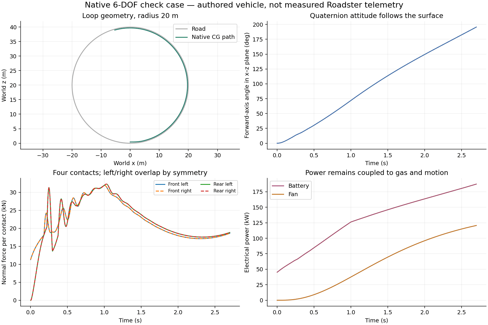
The new panel integrates world position and velocity, a scalar-first quaternion and three body angular rates. It evaluates m dv/dt = ΣF, I dω/dt = Σ(r × F) − ω × (Iω), and dq/dt = ½ q ⊗ [0,ω]. Coordinates are x forward, y left and z up. Principal inertias, CG, wheelbase, track, front steer, nozzle positions and force directions are explicit inputs. Each nozzle uses its share of the native group thrust, with the same nozzle count and tank state governing gas flow. NASA's rigid-body rotational-dynamics reference documents the quaternion/Euler formulation.
At each of four wheel points, signed road clearance sets a unilateral spring/damper force and bump-stop engagement. The normal is calculated from a plane, an inner circular cylinder (loop), or an outer cylinder (crest). Centripetal acceleration follows from world-frame motion and contact geometry. Per-wheel longitudinal and lateral force share one friction circle. Contact forces and the four gap-dependent suction patches each produce body moments. Wheel-point power feeds the inverter and shared DC budget, including regeneration and the measured battery voltage headroom.
The implementation checks cover ballistic fall, analytical offset-nozzle torque, torque-free energy/angular-momentum invariants, four-contact equilibrium and load transfer, curved contact through inversion, friction limits, gas conservation, battery limits, export round trips and step refinement. The illustrated loop uses authored mass properties and a 15 m/s initial speed. It reaches inversion but engages the bump stops and exceeds the entered total contact-load limit. It is a numerical check case, not a feasible manoeuvre or a reconstruction controller. Unsprung masses, wheel spin, body collisions, changing inertia and structural damage are outside this model.
6 · Measured battery response and its error
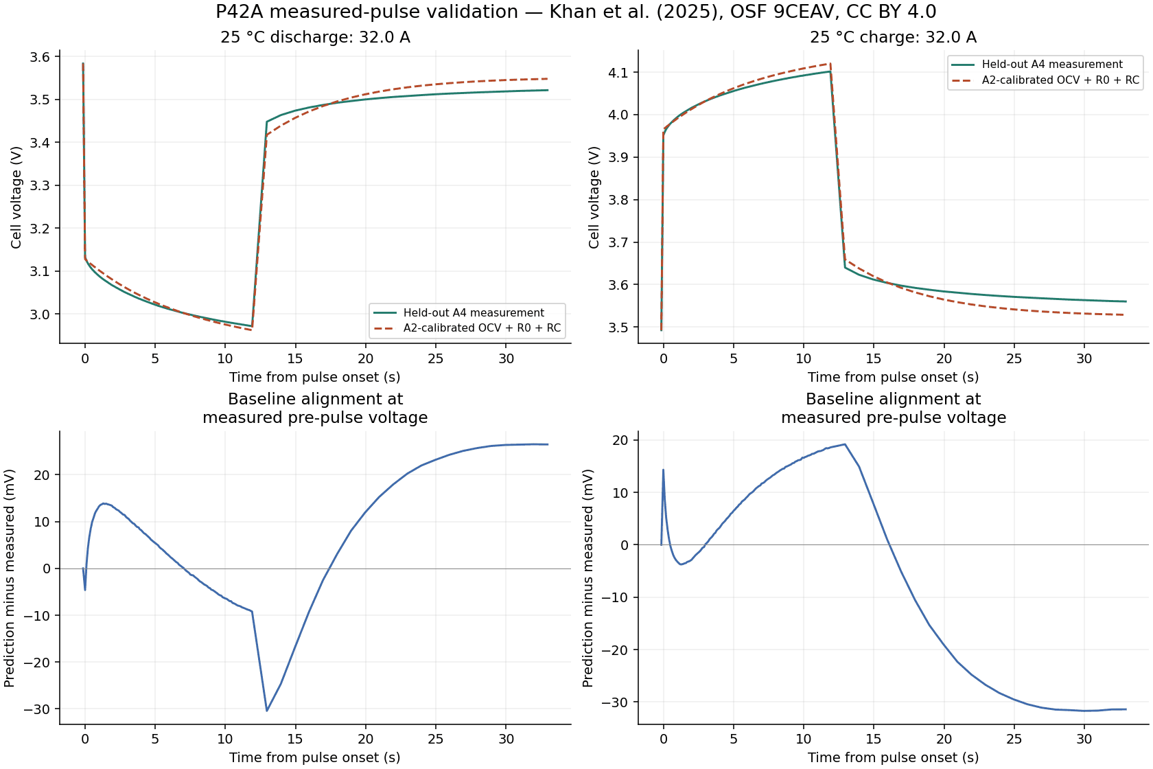
The profile buttons use Khan, Thatipamula, Tresca, Xu, Trewartha and Onori (2025), Scientific Data 12, 1506 and their OSF P42A dataset, licensed CC BY 4.0. The source archive retains download URLs, hashes, the exact selected samples, processing script and error reports. Rest OCV uses the authors' actual coulomb-counted SOC coordinates; nominal test-step labels are not substituted. Capacity comes from the training cell's C/20 discharge. Paired 0.5C pulse estimates supply R0(SOC), and a single R1/τ pair is fitted per temperature to cell A2's pulses and recovery.
| Temperature | Train / held out | Held-out windows | Pulse RMS / maximum error | Rest OCV RMS error |
|---|---|---|---|---|
| 5 °C chamber / 6.57 °C cell | A2 / A6 | 51 | 65.90 / 266.37 mV | 3.68 mV |
| 25 °C chamber / 25.17 °C cell | A2 / A4 | 65 | 11.20 / 48.90 mV | 3.72 mV |
| 40 °C chamber / 39.35 °C cell | A2 / A4 | 63 | 11.46 / 44.42 mV | 0.82 mV |
Pulse errors align each window to its measured pre-pulse voltage, then integrate measured current with the training-cell capacity and fitted RC model. They measure incremental pulse response; the separate rest-OCV error checks absolute OCV across cells. Only windows contained in the common measured SOC domain enter these statistics. Cell A4 in the nominal 5 °C cohort was actually near 12.7 °C, so the cold comparison uses thermally comparable A6 at 6.39 °C, selected on temperature. The remaining cold-cell error is reported, not hidden by retuning to the held-out data. Six representative held-out charge/discharge traces also run through the production native battery subgraph and agree with the fitted predictions within 0.05 mV.
Profile selection applies measured capacity, OCV, R0 and RC parameters, uses the measured reference temperature, and disables the extra authored temperature coefficient. The three profiles are separate temperature datasets, not an identified continuous temperature map. Initial conditions outside their stated SOC/temperature range are refused. Enforced operation derates over the final 0.1 percentage point of SOC and 0.5 °C inside the relevant calibration boundaries to avoid numerical on/off chatter.
The charge-pulse table retains observed current, SOC, duration and peak voltage. A roughly 13 s laboratory charge pulse does not establish a repeatable safe regeneration limit. The current cap remains a separately selected policy, defaulting to standard datasheet charging, while the native voltage cap uses measured OCV/R0 and the evolving RC state. The P42A data are not measurements of a Roadster cell or pack.
Measured profiles and validation metadata · Complete engineering correction source and evidence
Run the event on Lemonergy parts
Use the interactive study above to answer one design question: what does a thruster-and-suction event cost the battery, and which Lemonergy part limits it first? The road, scene, graphs and block diagram share one native Lemonergy run on the vehicle, propulsion and electrical blocks of catalog 2026.10. You can change every control directly in this wiki page without signing in.
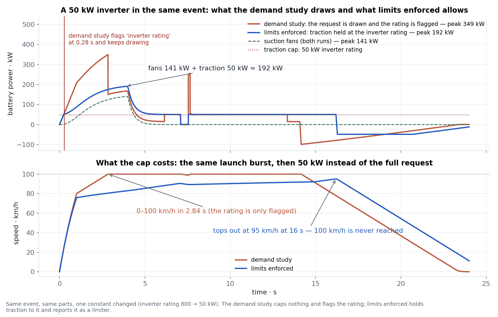
- Pick the study mode. Limits enforced (the default) caps what the model may draw at the inverter rating, the cells' and chain's current ratings, the terminal-voltage floor and ceiling, the SOC floor and the cells' temperature windows, and reports every active cap as a limiter. Demand study caps nothing and flags every exceedance, so you can see what an event would ask of parts that cannot deliver it.
- Choose a cell from the Designer library. The note under the picker states the record's basis and which fields are library estimates. Set Ns and Np; the pack line reports nominal voltage, capacity, energy, the pack mass with the Designer's fitted parts, the contactor and fuse chain rating, and a static check of the full-charge voltage against the chain parts' voltage rating.
- Keep Baseline as a comparison, then change the pedal acceleration, target speed or starting SOC. The driver command is a request; achieved motion comes from the solved forces, and starting SOC now changes the open-circuit voltage, the current and the terminal voltage.
- Open Battery model for ambient, initial pack temperature, cooling, the resistance temperature coefficient, the OCV end point and the SOC floor; Thrusters & gas for the nozzle split, thrust per nozzle and exhaust velocity at full tank, the tank blow-down law, burst timing and loaded gas (thrust falls with reservoir pressure and stops at regulator dropout or the choked-flow model boundary); Fans & suction for the suction level, fan operating point and spin-up time; Suspension & landing for ride frequency, damping, bump travel, bump-stop stiffness and the landing load limit; and Compressor refill to refill the tank from the battery after the run.
- In Make the road, edit section length and grade or add sections. A grade of 6% means 6 m rise per 100 m horizontal distance.
- Choose Play event, scrub Time, or move over a graph. The scene shows thrust, suction and airborne states at the same solver time as the graph cursors; the cursor table lists the road-load terms, the open-circuit and terminal voltages, the pack temperature, the suspension compression and what is limiting at that instant.
- Read the metrics together: event electricity, gas used and the electricity to restore it stand side by side with the total to repeat the event; the landing line gives impact speed, landing energy and peak load; the suspension line gives the maximum compression against the travel.
- Expand Inspect the connected Lemonergy blocks and Parts record for this run, then download the exact model, results CSV and run record before changing the candidate. The diagram opens as thirteen subsystem blocks — tank and thrust, suspension, battery, limits and so on — joined by the signals that cross between them; open a subsystem to see its blocks, with the signals it takes from the others as boundary blocks, or show every block on one canvas.
An orange status names the first sampled exceedance. With limits enforced that can only be physical or static — tyre grip is a limiter, the landing load limit, suspension bottom-out, exhausted gas, or a static voltage incompatibility of the chosen parts — because the electrical demand is held within the ratings and reported as limiters (traction cap, regeneration cap). In the demand study the same status reports the inverter rating, cell discharge rating or selected charge-current cap, the contactor and fuse rating, the terminal-voltage floor or ceiling, the cell temperature windows, the SOC floor and the battery power limit as they are exceeded, and later points remain hypothetical demand. Red dashed lines mark the first exceedance; the cell-current plot marks the selected record's continuous rating and the grip plot marks zero reserve.
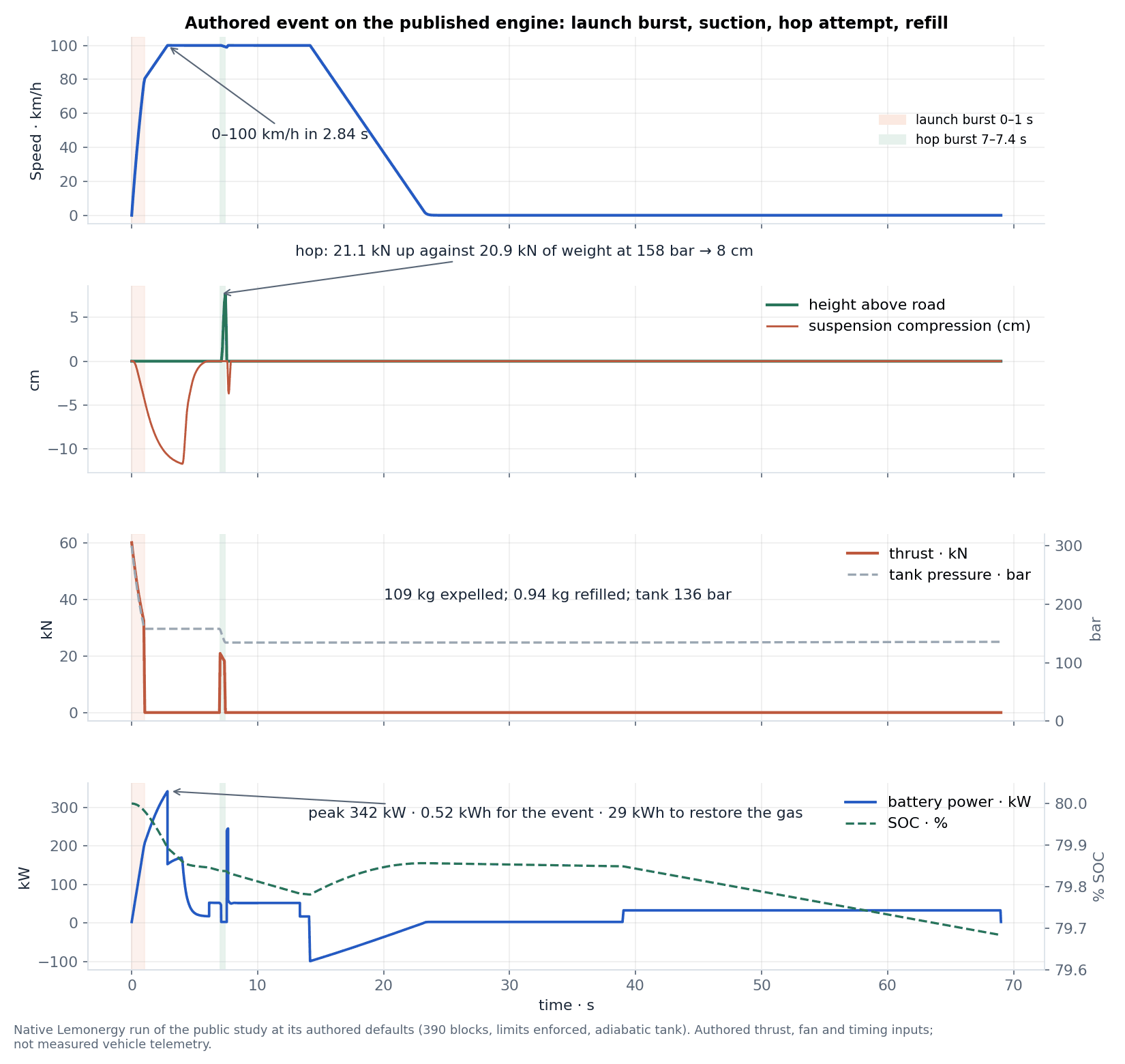
The figure is the default run drawn from its retained trace: the launch burst gives 0–100 km/h in 2.84 s while the thrust falls from 60 kN with the tank pressure; the hop at 158 bar lifts 21.1 kN against 20.9 kN of weight and only unloads the wheels; the battery peaks at 342 kW and spends 0.52 kWh, against 29 kWh to put the gas back. Every figure on this page is drawn from the retained native runs in verification/road-battery/road-battery-run.json and road-battery-results.csv, shipped in the source archive under Download the wiki source; run.mjs regenerates them from the published engine and figures.py redraws the figures. Your own run's data leaves the page through results CSV and run record, and the diagram's model through Download Lemonergy model.
Drive it yourself
Drive it yourself runs the same parts and the same blocks live — 380 blocks in the default drive and 390 in the default prepared event; imported calibration tables add native blocks, with nothing computed beside the engine except the display scaling. Releasing the pedal coasts: road load slows the car and no traction power is drawn. Hold speed (K) switches to the prepared event's driver law, which compensates road load so the car holds its speed uphill and draws the power that takes. Choose Start driving, then hold the pedal (W or ↑), brake (S or ↓), fire the forward thrusters (Space) or the upward nozzles (J), and switch the fans (F) and the compressor (C); on a phone, hold or tap the buttons under the frame. The studio frame shows the physics as it happens: the camera follows the car; the forces on the car inset draws weight, ground normal, suction, thrust, tyre and road-load forces from the step's block outputs, to one scale, with their values in kilonewtons; the live physics column writes the governing equations with that step's numbers substituted — tangential and normal balances, the longitudinal friction limit with its reserve, the road-load terms, the fan affinity law, the thruster mass flow, the battery power sum and the charge rate; the stopwatch blocks time 0–100 km/h, 0–60 mph and 400 m from the first movement; and the readout strip and strip charts keep the last 20 seconds. The block diagram under the frame can show the prepared event's blocks or the last drive rebuilt as one model. A red readout is a limit the selected Lemonergy part cannot meet: the trace reports any remaining physical or calibration exceedance. Electrical limits bind in Limits enforced mode; Demand study deliberately leaves electrical requests uncapped.
Record video (or V) captures that frame as a video file while you drive — WebM in Chrome, Edge and Firefox, MP4 in recent Safari — so a run can be shared with the forces and equations in it. The recording is the canvas as drawn; nothing is rendered separately for the file.
How it works: the drive is a co-simulation with a fixed 50 ms communication step. Your controls are constant sources for one step; the native engine integrates the plant over that step with the same Dormand–Prince 4(5) solver and tolerances as the prepared event, and the ten integrator states (speed, distance, height, normal speed, position, gas, SOC and energy counters) carry into the next step. The authored schedules, braking latch and target speed of the prepared event are replaced by your commands; the full pedal requests the pedal acceleration set in Driving & battery, the brake tapers to rest the same way as the authored brake, and the road continues flat beyond the authored sections. Nothing else changes: the road load, tyre-grip circle, thruster, fan-suction, suspension, battery, limit and converter-loss blocks are the same instances, and the study mode applies to the drive as well.
A drive is recorded as the times at which a control changed. Export this drive as a Lemonergy model writes those changes as Step sources on the same plant so the whole drive runs as one continuous model from the start, and Replay check runs that model in the engine and reports the largest difference from what you drove, sampled at every live step. The replay reports sampled differences. The live and replay plants use a maximum 5 ms internal step within each 50 ms communication interval; interpolation and contact events can contribute to the displayed deviation. Download drive CSV retains the live trace with your commands and the limit flags per step.
Choose the parts and their provenance
Every component value in the live model comes from a pinned Lemonergy parts snapshot generated from the Designer library, the Garage ledger and the open battery-data records. The snapshot records the Designer source revision, the battery-data commit and the SHA-256 of every file it read. Each record keeps its own provenance fields; a library estimate is labelled as one and a datasheet rating is never relabelled as a measurement.
| Part | Lemonergy source | What the study uses | Provenance carried |
|---|---|---|---|
| Cell (default Molicel INR21700-P42A) | Designer cell library | Capacity, nominal, charge and cut-off voltages, continuous discharge and standard charge currents, mass, DC resistance (16 mΩ at 10 A / 1 s), discharge window −40 to 60 °C, charge window 0 to 45 °C | Basis external_datasheet; estimated fields dims, priceUSD; source note. The record was corrected on 18 October 2026 from the datasheet (charge window, DC resistance basis, charge-current meaning); the 4.2 A charge figure is the standard CC-CV current, not a regeneration pulse rating |
| Alternative cells | Designer cell library; battery-data where contributed | Same fields; the Tesla 4680 and 2170 records are teardown-derived with every field estimated | Basis, estimated fields, record path and blob for contributed records |
| Pack mass | Garage ledger at the snapshot topology | Cells × 1.02 plus fitted busbar, holder, cooling, interface, heater and housing masses | Component ids and names from the Designer component database |
| Main contactor | battery-data component/te-connectivity/ev200aaana | 500 A continuous carry at 85 °C, 900 V; two per chain | Datasheet page and section locators; contact resistance from the Designer shelf class |
| Fuse | battery-data component/mersen/15nh3lgbat500 | 500 A, 1500 V gBAT link; one per chain | Datasheet page and section locators; resistance from the Designer shelf class |
| Interconnect lump | Designer architecture rule | 20 mΩ typical automotive busbar, joint and shunt lump | Rule text retained in the parts record |
| Traction inverter | Designer power-electronics class | Fixed, conduction and switching loss fractions at the stated rating | Class fractions retained in the parts record |
| Vehicle class and terrain | Designer EV class and terrain records | Drag area, rolling resistance, rotating mass, regeneration fraction, auxiliary load | Class values, editable |
The study still needs numbers that no Lemonergy record can supply. Nozzle count and loaded gas follow Tesla's public statements. Thrust per nozzle, effective exhaust velocity, the fan operating point, the compressor and the event timing are authored inputs, exposed so that they can be argued about.
| Quantity | Default | Unit | Basis |
|---|---|---|---|
| Nozzles | 10 | — | Tesla statement reported at the demonstration (InsideEVs) |
| Loaded gas | 250 | kg | Same statement; the tank pressure, temperature and volume were not stated |
| Suction at full fan | 2 | g of reference vehicle weight | "Up to 2 G" per Tesla's VP of Engineering, as reported; a media report of over 4,700 kg of downforce (Drive Tesla) is secondary |
| Thrust per nozzle at full tank | 10 | kN | Authored; Tesla states only that the thrusters exceed tyre force several times (Teslarati) |
| Effective exhaust velocity at full tank | 500 | m/s | Authored cold-gas value in the NASA thrust equation sense, lumping the pressure term |
| Tank blow-down | adiabatic, n = 1.4 | — | Polytropic reservoir sensitivity: n = 1.4 assumes negligible heat exchange during discharge; n = 1 assumes isothermal discharge. The n = 0 menu option selects a regulated nozzle rail with an adiabatic reservoir and pressure dropout. |
| Launch burst, hop burst | 1.0, 0.4 | s | Authored event timing |
| Fan operating point | 1.8 m², 4 m³/s, η 0.65 | — | Authored; the DOE fan-system sourcebook, printed page 6, explains why pressure, flow and efficiency belong together |
| Compressor | 30 kW, η 0.5, 300 bar | — | Authored; Tesla says the tanks can be refilled with compressed air but gives no rate |
| Vehicle mass without pack and gas | 1150 | kg | Authored; Tesla has published no mass |
| Fan spin-up time constant | 1 | s | Authored first-order lag; a step in suction would slam the suspension onto its bump stops |
| OCV at 0 % SOC | nominal − (max − nominal) per cell (3.0 V for the P42A) | V | Study assumption; the records carry nominal, charge and cut-off voltages but no OCV table |
| Resistance temperature coefficient | 0.02 | per K below 25 °C | Study assumption, bounded to 0.3–5× the 25 °C value |
| Pack heat capacity, cooling, ambient | cell mass × 1000 J/(kg·K), 800 W/K, 25 °C | — | Study assumptions; the records carry no thermal data |
| Suspension | 2.0 Hz ride frequency, ζ 0.4, 120 mm bump travel, bump stop 10× spring | — | Authored sports-car values; sprung mass only |
| Landing load limit | 3 | × weight | Authored study limit for the landing flag |
With the defaults the pack is 200s50p, 720 V nominal, 210 Ah, 151.2 kWh by nominal voltage × capacity, and 826 kg with the Designer's fitted parts (700 kg of cells). The vehicle is 2,226 kg with its gas. That pack mass is the first thing the Lemonergy ledger changes compared with an authored "2,000 kg including the pack": ten thousand 21700 cells weigh what they weigh.
Storage feasibility. The default 250 kg reservoir at 300 bar and 293.15 K requires about 701 L of internal volume for Z = 1. Real-gas compressibility is an explicit input. Vessel dry mass is added to the vehicle; a zero mass or envelope entry means unknown. Internal volume exceeding a supplied envelope fails a static check. Fitting the gas volume alone does not validate walls, fittings or structural pressure rating. Compressor energy remains a fixed final-pressure isothermal operating-point estimate, not an identified delivery/thermal map.
Equations and connected blocks
Positive current means discharge. Time is in seconds and every signal carries its SI quantity: speeds in m/s, forces in N, masses in kg, mass flows in kg/s, accelerations in m/s², powers in W. The model is built from the Lemonergy block catalog 2026.10, which adds the quantities and the vehicle, propulsion and math blocks this study needs, so the diagram reads as engineering rather than as a page of scaled Products. Motion is solved in the road frame of the current section: tangential coordinate s, speed v, height above the surface z and normal speed w. The road angle is θ = atan(grade / 100) and switches by distance through Compare blocks, so an event that changes the timing never shifts a hill.
Gas, tank and mass. For unregulated discharge, the tank blows down as it empties. For a polytropic tank the pressure follows the gas left, p/p₀ = (m/m₀)ⁿ, and the temperature T/T₀ = (m/m₀)^(n−1); a choked nozzle's thrust follows the chamber pressure and its exhaust velocity √T, so the mass flow ṁ = T/vₑ follows (m/m₀)^((n+1)/2). The thrust and exhaust velocity typed in are the full-tank values; a Divide and a Limit give the fill m/m₀, three Power-law blocks give the pressure ratio, the flow ratio and the exhaust velocity, and Products scale the commanded nozzle count by those ratios. A Cold-gas thruster block then turns the scaled nozzle count and the pressure/inventory gas-available flag into thrust (mode 0) or the mass flow that thrust costs (mode 1); the Integrator of refill minus thrust flow is the gas in the tank, and the total mass is the vehicle with its pack plus that gas:
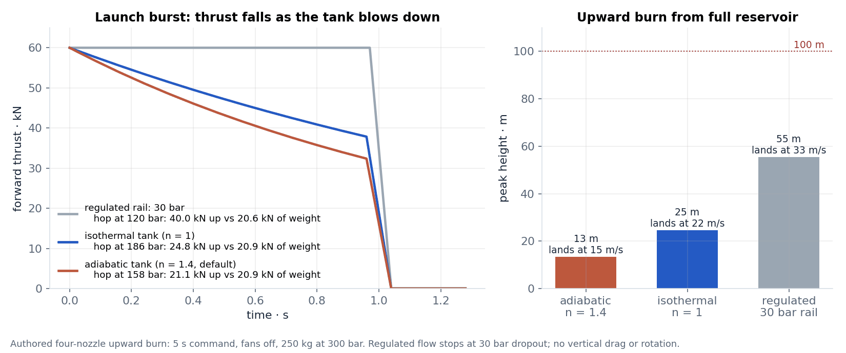
The unregulated reservoir uses p/p_full = (m/m_full)^n, with n = 1.4 for an adiabatic sensitivity and n = 1 for isothermal. Selecting regulated supply holds the authored nozzle thrust while the reservoir continues to blow down adiabatically. The default delivery rail is 30 bar; the nozzles stop at dropout, retaining about 48 kg of unusable reservoir gas. Unregulated thrust is not extrapolated below the 1.89 bar absolute cutoff of the choked-flow approximation at 1 bar ambient, using the ideal-air critical pressure ratio from the NASA choked-flow relations. Regulated thrust is a separately authored nozzle operating point at the delivery rail; equal thrust does not imply the same nozzle geometry at 30 and 300 bar. With the authored four-nozzle upward burn the corrected model reaches approximately 13 m adiabatic, 25 m isothermal and 55 m regulated. These are sensitivity results for chosen inputs, not bounds on the actual Roadster. No reservoir energy balance during refill, nozzle geometry identification or vertical aerodynamic drag is solved.
Suction and seal opening. A quasi-steady parabolic fan curve is intersected with an orifice-style leakage curve. Let h = max(0, body rise − seal compliance), u = (h / leakage gap scale)², k_p = 1/(1 + u/2), and k_Q = sqrt((1 + u)/(1 + u/2)). The electrical operating-point factor is k_P = free-flow fraction + (1 − free-flow fraction) k_p k_Q. The native outputs are F_s = F_reference f² k_p, P_fan = P_reference f³ k_P, Q = Q_reference f k_Q and Δp = F_s / area. When the gap opens, adhesion tends toward zero while free-flow power remains. The same operating-point power is used by the battery allocator. The curve, seal compliance and gap scale are authored sensitivities that need measured fan/seal data.
Fixed hardware is the default comparison mode: changing the cell or parallel count does not resize fan force/power ratings, spring stiffness or damping. The reference vehicle mass is explicit. Actual ride frequency changes with candidate mass. The optional resize mode is an explicit hardware redesign. Suspension preload defines the loaded equilibrium; supplied bump travel is measured from that equilibrium.
Suspension and contact. The body rides on an explicit sprung-mass suspension along the road normal: z is the body height above the loaded ride height, the spring is preloaded to the loaded weight, a damper acts while the wheels touch, a bump stop takes over beyond the bump travel, and the wheels leave the road when the spring force would reach zero (the droop travel). The ground can only push:
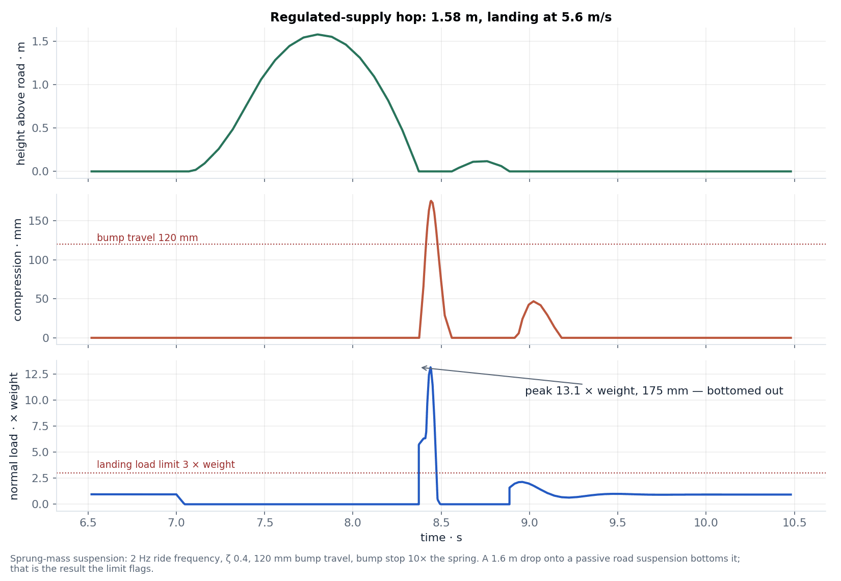
ω₀ = 2π × reference ride frequency. In the stiffness and damping formulas, m₀ is the hardware reference mass; preload and droop use the candidate loaded mass instead; s_bump is the bump travel. Height above the road is max(0, z − z_droop); compression is max(0, −z). The bump stop engaging is flagged as suspension bottom-out and a normal load above the landing load limit as landing load limit; the metrics report the impact speed, ½m w², the peak load and the maximum compression. Two g of suction alone compresses the default suspension to its bump stop, and a landing from the 1.5 m hop of the regulated-supply scenario onto a passive road suspension bottoms it hard — those are results, not artefacts, and the inputs let you try a stiffer or longer-travel suspension. Sprung mass only: no unsprung mass, tyre spring or rotation.
Road load, driver and tyres. The Road-load block is the Designer vehicle rule in newtons; the Tyre-grip block is the longitudinal friction limit on the positive normal force:
The three road-load terms are also built from primitive blocks — a Minimum/maximum for max(0, N), two Compares and a Sum for sign(v)·[|v| > 0.1 m/s], an Absolute and Products for v|v| and m g sin θ — and summed; the Sum of those terms minus the Road-load block is the road-load-residual signal, which the tests require to be zero at every point. Each term is therefore inspectable in the diagram and in the exported model, and the live frame reads them as block outputs rather than recomputing them.
The stopwatches are blocks too. A flag such as v ≥ 100 km/h is a Compare; its Integrator never returns to zero once the flag has been true, so a Compare on that integral is a latch without any sampled block, and it carries across the drive's communication steps like every other integrator. The time from first movement to the mark is the Integrator of has-moved × (1 − reached):
The pedal accelerates until the target speed, cruises, and brakes from the distance L − v² / (2 a_cmd) (a Power-law block on the speed) through a sampled Boolean latch (0.04 s); braking tapers over the last 0.2 s × a_cmd of speed so the car settles at rest. The achieved motion is grip-limited, and the grip reserve μN − |F_request| (an Absolute block) is the reported margin.
Electrical. Minimum/maximum blocks split the tyre force into drive and braking parts; the Converter-loss block is the Designer power-electronics class on the throughput; the fans, the compressor and the auxiliaries add to the demand:
Battery. The default OCV curve and resistance temperature coefficient remain assumptions. Optional source-labelled JSON supplies a cell-specific OCV(SOC) table, R0(SOC) table at a stated reference temperature, and a one-RC polarisation branch. Tables cover their declared SOC domain with piecewise-linear native blocks; without a declared domain they must cover 0–1. Initial conditions outside calibration validity are refused, and enforced operation derates at the boundaries. A supplied cellId must match the chosen cell, a test/source reference is mandatory, and its temperature tolerance is retained and enforced. Lemonergy records the source without declaring uploaded data independently validated.
U = OCV(SOC) − V_RC; I = 2P_dc / (U + sqrt(U² − 4 R P_dc)); V_terminal = U − I R
dV_RC/dt = (I R1 − V_RC)/τ; dSOC/dt = −I/(3600 Q)
R = R_cells(SOC,T) + R_chain; C dT/dt = I²R_cells + V_RC²/R1 − G(T − T_ambient)
The RC branch is disabled when no parameters are supplied. Chain heat I²R_chain is retained as an electrical loss and reported separately, rather than deposited into the cell thermal mass. The selected charge cap defaults to the datasheet standard CC-CV current; it is a conservative study policy, not a verified maximum regenerative pulse rating. The thermal coefficient, heat capacity and cooling remain authored inputs unless separately identified.
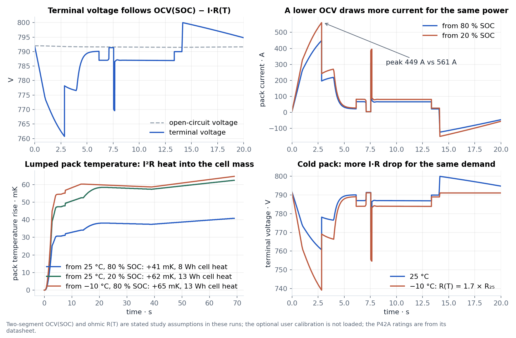
Limits. Both modes share one native plant. In Limits enforced mode, the permitted current is max(0, min(cell current rating × Np, chain current rating, (OCV − Vmin)/R, OCV/(2R))). This keeps the power cap on the stable, low-current branch of the ohmic battery model. The resulting terminal-power budget is zero outside the discharge temperature window and tapers over the last 0.1 percentage point above the SOC floor. The study allocates that budget in this explicit order: auxiliaries, inverter idle, fans, compressor, then traction. This is a study policy, not an identified Tesla BMS strategy. Fan operating fraction is capped by the cube root of the power available to it; compressor mass flow scales with the delivered electrical power. Active fan, compressor, auxiliary, traction and regeneration caps are reported separately. Regeneration also respects the chain current rating. The voltage and charge-window caps remain:
With limits enforced, every battery-fed load shares the feasible bus allocation, including inverter idle and auxiliaries. A fan power cap also reduces suction; a compressor cap reduces the refill rate. With no discharge permission the bus draws no residual idle power. Demand study retains the uncapped request and its exceedance flags. The allocation and its effects are part of the downloaded native model, live-drive replay and CSV.
| Native block group | Lemonergy blocks | Signals to inspect |
|---|---|---|
| Schedules | Step pairs for launch, hop, fan and compressor windows | launch-window, hop-window, fan-window, refill-window |
| Gas and mass | Cold-gas thruster (thrust and mass-flow modes), Compare gates, gas Integrator, mass Sum | gas-mass, mass, thrust-forward, thrust-up, thrust-flow |
| Tank blow-down | Divide and Limit for the fill m/m₀; Power-law blocks for (m/m₀)ⁿ, (m/m₀)^((n+1)/2) and vₑ; Gain for the pressure in pascals; Products that scale the commanded nozzles | tank-fill, tank-pressure-ratio, tank-pressure, thrust-flow-ratio, exhaust-velocity, hop-nozzles-thrust |
| Road | Distance Compares → grade Gains → sine and cosine Sums | grade-sine, grade-cosine |
| Suction | Suction fan in power and force modes | fan-command, fan-power, suction-force |
| Suspension | Preload Constant, −k·z Gain, bump-stop Minimum/maximum and Gain, damper Gain, droop Compare, wheel-force Sum and Minimum/maximum, Product with contact → normal Integrators | spring-force, bump-stop-force, damper-force, normal-force, height, compression, contact, bottomed |
| Driver and tyres | Road load, target-speed Compare, Power-law stop distance, Boolean latch, pedal Sum, Tyre grip, Absolute, Divide (grip reserve fraction) | road-load, pedal, tyre-request, tyre-force, grip-margin, grip-reserve |
| Road-load terms | Minimum/maximum, Compares and Sum for sign(v), Products for rolling, drag and grade, a Sum and a residual Sum against the Road-load block | rolling-force, drag-force, grade-force, road-load-residual |
| Stopwatches | Compare flags → Integrators that latch (a flag's integral never returns to zero) → Products and Integrators that count from first movement | has-moved, reached-100kph, t-100kph, t-60mph, t-400m |
| Motion | Net force Sum → Divide by mass → speed Integrator → distance and world-position Integrators | speed, distance, x-position, y-position |
| Electrical | Minimum/maximum splits, Products, Converter loss, fan, compressor and auxiliary Sums | motor-power, inverter-loss, traction-dc, battery-power |
| Battery | Select between two OCV Gains on SOC; Limit on 1 + α(25 − T) and a Gain for R(T); Power-law for OCV² and √; Sums, Divide for the current; Product for V_t·I; Gain −1/(3600Q) → SOC Integrator; Thermal rate → temperature Integrator | ocv, resistance, discriminant, battery-current, terminal-voltage, cell-current, soc, pack-temperature, ohmic-heat |
| Limits | Products and Divides for the power at each rating, Minimum/maximum chains, Compares for the SOC and temperature gates, Selects on the mode constant, Divide for the force cap, Minimum/maximum on the request | p-at-idis, p-at-vmin, traction-cap, force-cap, traction-limited, regen-cap, regen-limited, battery-feasible |
| Energy to repeat | Gas-deficit Sum and a Gain at the compressor's electrical cost per kilogram | gas-used, restore-energy |
Every block belongs to one of thirteen subsystems (constants and schedules, tank and thrust, road geometry, limits, suction fans, suspension and contact, driver and tyres, road-load terms, stopwatches, motion, electrical, battery, energy to repeat). The exported model carries the membership on each block and the list on the graph as drawing hints — the engine runs the flat graph — and the diagram uses them for its overview, its drill-down and the bands of the flat canvas.
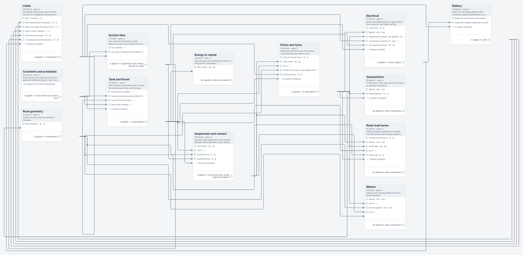
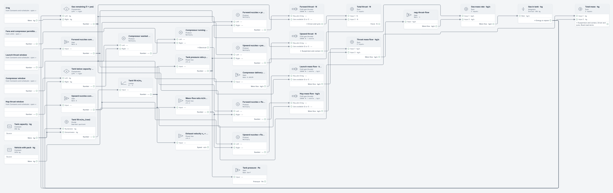
Every block above is a type of the Lemonergy block catalog 2026.10, which this wiki ships and runs: 21 types, 390 blocks in the default event and 380 in the default drive; calibration tables and the optional RC branch add native blocks, nothing bespoke. The exported model round-trips through the Studio file format with its checksum, and the tests rerun it from the file. The authenticated Pro editor at design.lemonergy.com runs the same catalog (2026.10.1), so the downloaded model opens, rewires and runs there with the same checksum; the editor's own test reruns this study's baseline from the exported file. When the selected cell has a battery-data record with page locators, the bus-voltage and coulomb-counting blocks carry a component-binding with the record's commit, blob and evidence identifiers; the inspector shows it.
Rebuild the model step by step
The model is built in the order below, one subsystem per step, and each step can be checked on its own before the next is wired. Use Inspect the connected Lemonergy blocks to see the subsystems and, inside each, every block and connection of the prepared event, and Download Lemonergy model to compare your graph with the file; the signal names are the block ids in that file. Every signal carries an SI quantity, and a block refuses an input of the wrong quantity, so the catalog itself checks the wiring.
- Constants and schedules. Constant blocks for the masses, ratings and authored inputs (
dry-mass,tank-capacity,limits-enforced, the cell ratings); Step pairs summed into the launch, hop, fan and compressor windows (launch-window= Step on − Step off). Check: each window is 1 inside its interval and 0 outside. - Tank and thrust. Gain blocks turn a window into commanded nozzles (
launch-nozzles= 6 × window); Divide the gas Integrator by the tank capacity and Limit it to 0–2 (tank-fill); Power-law blocks give (m/m₀)ⁿ, (m/m₀)^((n+1)/2) and vₑ₀ (m/m₀)^((n−1)/2); Products scale the nozzles; two Cold-gas thruster blocks per direction give thrust (mode 0) and mass flow (mode 1) from the scaled nozzles and the Comparegas-available; a Sum of refill minus thrust flow feeds the gas Integrator (initial 250 kg), and a Sum with the dry mass is the total mass. Check: at full tank the thrust is nozzles × T₁ and ṁ = T / vₑ; the Regulated gas supply scenario holds the authored nozzle operating point only above dropout. Separate Integrators retain gross gas expelled and refilled; a nonnegative deficit drives remaining refill energy. - Road geometry. Compares on the distance Integrator against each section start, Gains for the change in sin θ and cos θ, and Sums give
grade-sineandgrade-cosine. Check: sin θ steps from 0 to 0.0599 at 150 m on the default road. - Suspension and contact. A Constant preload m₀g, a Gain −k on the height Integrator, a Minimum/maximum and Gain for the bump stop, a Gain −c on the normal-speed Integrator, a Sum for the wheel force, a Minimum/maximum against zero, a Compare for contact (z ≤ z_droop) and a Product give
normal-force; the normal balance Sum over the mass (Divide) feeds the normal-speed and height Integrators. Check: at rest the normal force is one weight and the compression zero; with 2 g of suction the spring reaches its bump stop. - Suction. The fan target and first-order spin-up feed the battery-budget cap. Native blocks compute gap-dependent pressure, flow and operating-point power factors from body rise and seal compliance. Suction-fan outputs are multiplied by the same factors used in the electrical allocation. Check: F = F_reference f² k_p and P = P_reference f³ k_P at every retained point; opening the seal removes adhesion.
- Driver and tyres. Road load from the Road-load block on the normal force, speed, mass and grade; the pedal law from a Compare on the target speed, a Power-law stop distance and a Boolean latch; the request Sum; the Tyre-grip block on the request and the normal force; an Absolute and a Divide for the grip reserve. The road-load terms are rebuilt from primitives and the residual Sum against the Road-load block must be zero. Check: at 100 km/h on a flat road with the fans off the terms are about 0.21 kN rolling (Crr × one weight), 0.30 kN drag and 0 kN grade; with 2 g of suction the rolling term triples because it acts on the normal load.
- Motion. The tangential Sum of tyre force, forward thrust and road load, a Divide by m(1 + ε), the speed Integrator, the distance Integrator and the world-position Integrators (speed × cos θ and sin θ, plus the normal motion). Check: the Regulated gas supply launch matches the variable-mass closed form.
- Electrical. Minimum/maximum splits of the tyre power into motor and braking parts, the Converter-loss block on the throughput, the regeneration Gain and cap, and the Sum
battery-powerof motor, loss, fans, compressor and auxiliaries less regeneration. Check: the loss is the Designer class fractions applied to the throughput. - Battery. Assumed two-segment or supplied piecewise-linear tables give OCV(SOC) and R0(SOC). An optional First-order block solves RC polarisation. The stable quadratic current root uses U = OCV − V_RC, with separate cell and chain resistance. The SOC Integrator counts coulombs; cell ohmic and RC dissipation feed the cell thermal state, while chain heat is separate. Check: V_terminal I equals the allocated DC power on the feasible branch; integrated current equals the SOC change.
- Limits, stopwatches and energy. The cap chain of Products, Divides and Minimum/maximum blocks, the Compares for the SOC and temperature gates, the Selects on
limits-enforced; the stopwatch Compares and latching Integrators; gross gas-out/refill Integrators, the nonnegative gas-deficit calculation and the restore-energy Gain. Check: the 400 m stopwatch uses exactly 400 m; with limits enforced every DC load shares the feasible battery budget and tyre force never exceedsforce-cap; in the demand study the flags fire where the ratings are exceeded.
The drive uses the same graph with the schedules replaced by Constant sources for one 50 ms step; the exported drive replaces those constants with Step sources, so a recorded drive is the same recipe with a different schedule.
Compare engineering scenarios
Keep the baseline before using a scenario button. Each button restores the default road and inputs, then changes the stated input. With the default parts, limits enforced and the adiabatic tank, the run reports about 342 kW peak battery power, 9.0 A peak cell current against the P42A's 45 A rating, a terminal voltage between 761 and 800 V, 141 kW of fan power at 2 g of suction, a launch whose thrust falls from 60 kN as the tank blows down so that 0–100 km/h takes 2.8 s (0.9 s with a regulated supply), a hop that only unloads the wheels — 21.1 kN upward against 20.9 kN of weight with the tank at 158 bar after the launch burst, 8 cm, 0.3 s — 109 kg expelled, about 0.94 kg refilled, leaving the tank at 136 bar, 0.52 kWh of event electricity against 29 kWh and 58 minutes at 30 kW to restore the gas, and SOC falling from 80 % to 79.68 %. The thrust, not the battery, produces the launch; the gas, not the electricity, is the cost of repeating it; and the tank pressure, not the gas mass, decides whether the hop leaves the ground.
| Scenario | Controlled change | Expected engineering effect | Decision to carry forward |
|---|---|---|---|
| Demand study | Limits enforced → demand study | The same event with nothing capped: every rating the parts cannot meet is flagged at the instant it is exceeded | Read which part limits first before changing the parts |
| Hard acceleration | 3 → 10 m/s² pedal | Tyre power rises toward the grip limit; braking regeneration runs into the charge-current cap (enforced) or exceeds the selected charge-current policy (demand) | Check the selected charge cap and obtain pulse charge-acceptance data before relying on recovery |
| Low SOC | 80 → 10% initial SOC | Lower OCV, more current for the same power, lower terminal voltage; the floor and the SOC floor come closer | Set an operating SOC window; obtain a measured OCV table to replace the two-segment assumption |
| Cold pack −10 °C | Pack and ambient at −10 °C | Resistance 1.7× the 25 °C value: more I·R drop, more heat, lower terminal voltage; charging is outside the 0 °C charge window | Obtain resistance versus temperature and decide on pre-conditioning |
| Fans off | λ_max 0, fan fraction 0 | Normal load drops to one weight; grip reserve falls; fan power disappears | Decide what the suction buys per kilowatt |
| No thrust | 0 kN per nozzle | The pedal alone drives the car; no hop; gas untouched | Compare launch time with and without gas |
| Regulated gas supply | Unregulated → 30 bar regulated rail | Constant 60 kN launch (0–100 km/h in 0.9 s), a 1.6 m hop with 1.3 s airborne, a landing at 5.6 m/s (32 kJ) that bottoms the suspension at 13 × weight and is flagged, about 152 kg expelled | A regulator or a far larger tank would be needed for the authored event; decide which is being claimed |
| Vertical reserve: upward burn | Fans off; no launch; five-second upward command from full reservoir | About 13 m adiabatic, 25 m isothermal and 55 m regulated with the 30 bar rail; regulator dropout retains residual gas. Landing exceeds the chosen load limit. | Compare authored nozzle and storage assumptions. This model cannot establish actual Roadster flight capability or safe landing. |
| Fewer parallel cells | 50p → 25p | Lighter pack, about double per-cell current, higher ohmic drop | Check current rating, pack mass and cooling together |
| Tesla 4680 record | 195s9p teardown-derived cell | The selected 35 A placeholder limits discharge in enforced mode; demand mode flags requests above it | Replace the placeholder with a measured rating before any claim |
| Long refill | 300 s at 60 kW | The compressor becomes the dominant energy use | Decide whether refill belongs on the traction battery at all |
| Road grade | Flat versus climb or descent | Gravity changes tyre force, grip reserve and energy | Compare the same route length, speed and pack |
Parallel-cell count changes electrical capacity, current sharing, the loss estimate and the pack mass immediately, because the mass comes from the Designer ledger rather than a typed total. Hold dry mass, vessel mass and reference hardware fixed when comparing packs; change them explicitly when comparing vehicle redesigns.
The native solver is Dormand–Prince 4(5), relative tolerance 1e−7, absolute tolerance 1e−6 in SI units, and maximum step min(0.1 s, duration / 400). Schedules are explicit Step events; contact, bump stop, braking, gas, tank, SOC and temperature gates are Compare blocks solved with the dynamics. Numerical checks compare the launch and ballistic flight against analytical motion, verify the road-load, force, inverter-loss, power, affinity and coulomb balances at every point, and repeat with half the maximum step; the engine's own tests check each new block against its closed form, including a thrust launch against the variable-mass solution. These are implementation checks, not experimental vehicle validation. Peaks and violation times are sampled observations at the retained solver resolution.
Continue in the Designer and Simulation
Use Save run & parts record to retain the parts snapshot provenance, cell identity, Ns/Np, complete road, authored thrust, fan and compressor inputs, solver settings, graph checksum and native trace. This is the configuration record for the next design decision.
- Choose Open this pack in the Designer. The link carries the cell, Ns and Np in the Designer's own design-link format, so the Garage ledger starts from the same candidate.
- Compare the Garage pack mass and component ledger with the parts record of this run. The study scales the fitted parts from the snapshot topology; the Designer lays the pack out for the exact topology.
- Enter the vehicle mass without pack in the Designer's vehicle control. Add this study's dry vehicle mass and vessel dry mass for the Designer vehicle control; pack and gas remain separate here.
- Return with any changed cell or topology and compare against the retained baseline. Check current, SOC, grip, tank pressure, hop height and gas together.
- For full block editing, use Download Lemonergy model, then import the
.lemon.jsonfile into Co-Simulation Studio in the authenticated Design workspace, which runs the same catalog 2026.10.1 and opens the file with every vehicle, propulsion and math block in place. Inspect the imported graph before running it.
The wiki exports the precise model and inputs; automatic import of the complete event into the Garage is not yet released. The Designer link restores a candidate pack; it does not carry the road, thrust or fan inputs.
Extend the battery model with measured data
Coulomb counting needs an initial SOC, a capacity convention and accurate current. Movassagh et al. (2021), Energies 14, 4074 analyse the resulting error sources. Integration does not measure the initial SOC or correct an incorrect capacity.
The measured P42A buttons now supply capacity, OCV/R0 and fitted RC parameters with held-out validation, as documented in item 6 above. The calibration field also accepts other sourced tables and RC data matched to the selected cell, SOC, temperature and timescale; imported fields are carried into the model and run record. The default assumed curve is retained only when no table is supplied. Single-temperature data and a chosen temperature coefficient do not establish performance across the complete cell temperature range. The separate reference-cell example below remains an analytical circuit check, not a calibration of the chosen vehicle pack.
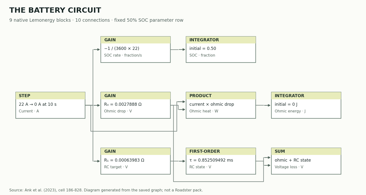
For a sourced dynamic reference, run the 4680 reference-cell circuit. Its nine existing blocks calculate SOC, ohmic voltage loss, an RC state and ohmic energy from a 22 A pulse. It uses Ank et al.'s paper and open dataset, first-generation Model Y cell 186-828, EIS parameter file at 50% SOC. It is a separate reference-cell check, not the live candidate pack or a new Roadster cell.
| Reference-cell input | Value | Basis |
|---|---|---|
| Capacity denominator | 22 Ah | Published nominal C-rate convention |
| Pulse | 22 A for 10 s | Authored test using the source protocol conditions |
| R0 | 0.0027888 Ω | Source EIS fit, 50% SOC |
| R1 | 0.00063983 Ω | Source EIS fit, 50% SOC |
| C1 | 1.3324 F | Source EIS fit; not converted from millifarads |
| R1 C1 | 0.000852509492 s | Derived time constant |
The retained run ends at 49.722222% SOC with 13.497792 J of ohmic energy. Seven analytical signal checks passed over 3,734 native solver points. These validate the implemented circuit equations, not physical pulse accuracy. No OCV map was supplied for that example, so its voltage output is a loss, not terminal voltage.
Reference-cell model · Run evidence · Results CSV
Extend contact, suction and gas scenarios
For a static orientation study, run the existing contact cases: μ = 0.5, μ = 1, or μ = 1.5. Each uses 28 native blocks to sweep suction/weight from 0 to 2 at five fixed orientations.
N/(mg) = λ + cos θ
static traction reserve/(mg) = μ(λ + cos θ) − |sin θ|
Both positive normal reaction and nonnegative reserve are required. The 0–1 s solver clock is a sweep coordinate, not driving time. These cases include wall and ceiling orientations but no curvature, suspension or free flight. Download the contact scenario evidence and comparison CSV.
The Tesla video and independent interactive concept motivate the fuller event modelled above. They do not supply a verified cell model, fan map, tank state or actuator allocation. BASENOR's battery discussion is a secondary source for reported pack claims, not a parameter-identification dataset.
| Subsystem | Status in the live model | Evidence needed before predicting performance |
|---|---|---|
| Four fan zones | Equivalent fan in the road/hop study; four separate seal patches with moments and shared power in the 6-DOF study | Pressure/flow maps, leakage, effective area and sealing transients |
| Gas inventory and nozzles | Polytropic reservoir, separate regulator rail and dropout, choked-flow cutoff, gross gas-out/refill accounting, required storage volume, manufacturer cylinder dimensions, derived vessel mass and dimensional packing checks | Tank volume, initial pressure and temperature, valve and regulator behaviour, wall heat transfer |
| Nozzle thrust | F = ṁ ve with an effective exhaust velocity lumping (pe − pamb)Ae, both scaled with the tank state | Nozzle geometry, thrust coefficient against pressure ratio and chamber conditions for the full NASA thrust equation |
| Hop and landing | Sprung-mass suspension with preload, damper, bump travel and bump stop; impact speed, landing energy and peak load reported | Unsprung mass and tyre spring, measured spring and damper curves, structural landing criteria |
| Battery | Published P42A capacity/OCV/R0/RC profiles with held-out errors, or explicit fallback/uploaded data; separate cell and chain heating; voltage and operating-window limits | Measured OCV table, impedance versus SOC and temperature, cell thermal network and cooling capacity |
| Rotation and barrel roll | Not modelled | Inertia tensor, nozzle positions and moment arms, control allocation |
| Compressor refill | Constant electrical load at an authored efficiency and isothermal work | Measured compressor power and delivery curve against tank pressure |
A tank volume alone does not determine gas mass or flight duration. With the default compressor inputs a full 250 kg refill costs about 67 kWh, 44% of the pack's nominal energy, and takes more than two hours at 30 kW: refilling is a between-runs matter, not a lap matter, unless the compressor is far larger than the authored value.
Record a reproducible demonstration
Keep the parts record and baseline overlay visible. Show the chosen cell and its provenance line, the road edit, the thrust or fan change, the resulting power, current, SOC, height and gas graphs, and any violated constraint. Inspect the exact connected blocks and finish with the saved model and the Designer link. Record the real Lemonergy interface after the scenario has been reviewed; animation should explain the engineering result.